Chapter 5 Random Variables and Probability Distributions
5.1 Why random variables?
A probability model initially describes outcomes such as claim/no claim, a sequence of coin tosses, or a measured lifetime. Numerical analysis becomes possible only after we translate each outcome into a number. That translation is the role of a random variable.
A random variable is a function \(X:S\to\mathbb{R}\) assigning a real number \(X(\omega)\) to every outcome \(\omega\) in the sample space \(S\). Its support is the set of values that can occur with positive probability or density.
The adjective random describes the input outcome, not the function. Once \(\omega\) is known, \(X(\omega)\) is fixed. Different experiments can also produce the same probability distribution—for example, a fair-coin payoff and an even/odd die payoff may have identical numerical values and probabilities.
5.2 Discrete random variables
\(X\) is discrete when its support is finite or countably infinite. Its probability mass function (pmf) is
\[p_X(x)=\mathbb{P}(X=x),\]
where \(p_X(x)\ge0\) and \(\sum_xp_X(x)=1\).
For an event described by a set \(A\),
\[\mathbb{P}(X\in A)=\sum_{x\in A}p_X(x).\]
Example: number of heads
Two fair coins are tossed and \(X\) counts heads. Its support is \(\{0,1,2\}\) and its pmf is \((1/4,1/2,1/4)\).
##   x probability
## 1 0        0.25
## 2 1        0.50
## 3 2        0.25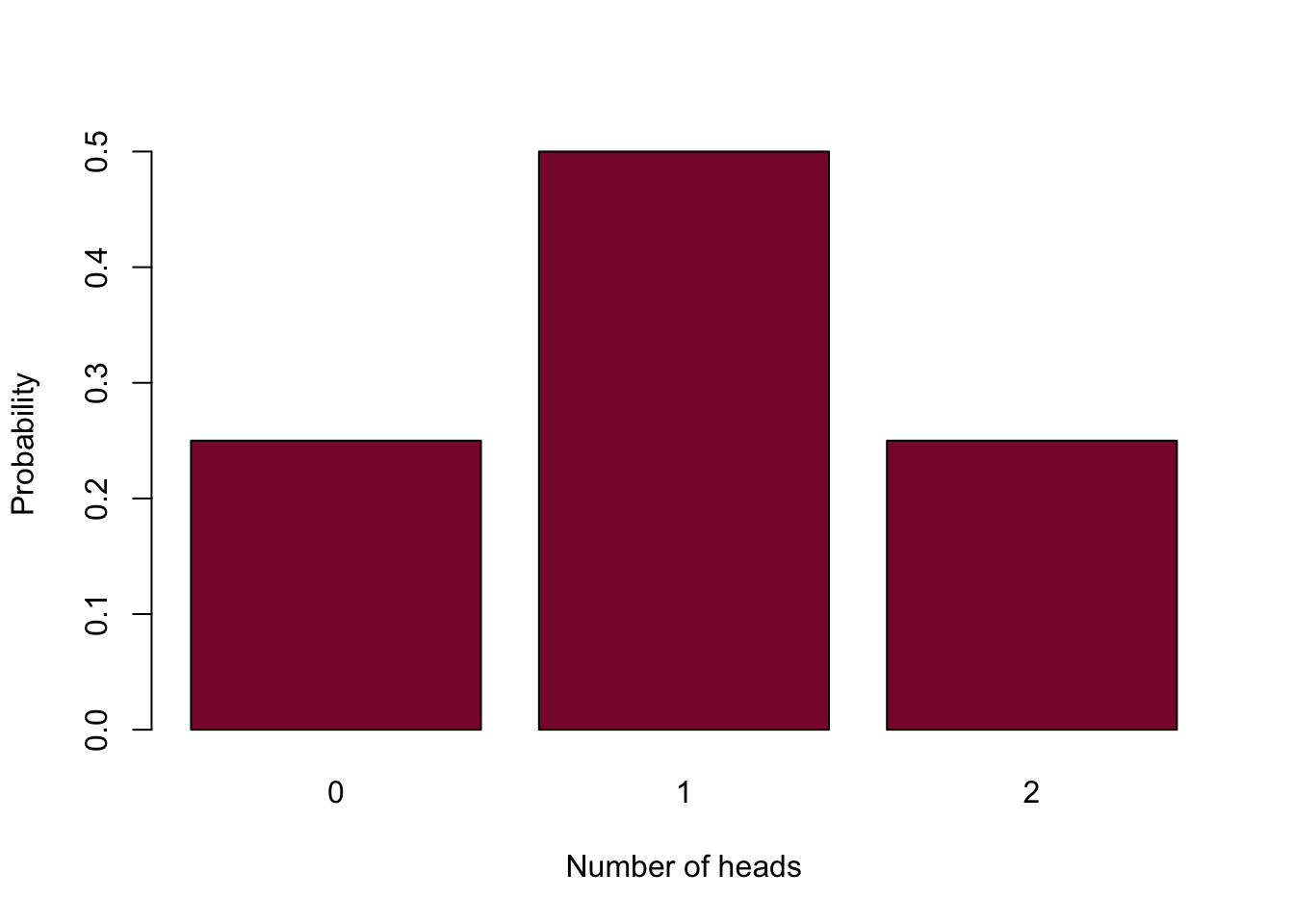
Example: constructing a pmf from proportional weights
A loaded die is designed so that face \(j\) has probability proportional to \(j\). Write \(p_X(j)=cj\) for \(j=1,\ldots,6\). The probabilities must total 1, so
\[c(1+2+3+4+5+6)=1\quad\Longrightarrow\quad c=\frac1{21}.\]
Therefore
\[\mathbb{P}(X\text{ is even})=p_X(2)+p_X(4)+p_X(6)=\frac{2+4+6}{21}=\frac47.\]
“Proportional to” determines the relative sizes of the probabilities but not their scale. The condition that probabilities sum to 1 supplies the missing normalizing constant.
##   face probability cumulative_probability
## 1    1  0.04761905             0.04761905
## 2    2  0.09523810             0.14285714
## 3    3  0.14285714             0.28571429
## 4    4  0.19047619             0.47619048
## 5    5  0.23809524             0.71428571
## 6 6 0.28571429 1.00000000## [1] 0.57142865.3 Continuous random variables
Discrete models place probability at points. Measurements such as time, severity, and return are usually modeled over intervals.
\(X\) is continuous when probabilities are generated by a probability density function (pdf) \(f_X\) satisfying
\[f_X(x)\ge0,\qquad \int_{-\infty}^{\infty}f_X(x)\,dx=1.\]
For \(a<b\),
\[\mathbb{P}(a<X\le b)=\int_a^b f_X(x)\,dx.\]
Density is not probability at a point: for a continuous variable, \(\mathbb{P}(X=x)=0\). Probability is area, so including or excluding an interval endpoint makes no difference. A density can exceed 1 provided its total area is 1.
Example: a triangular density
Let \(f(x)=2x\) on \(0<x<1\) and \(f(x)=0\) elsewhere. Before using the formula, verify that it is a density:
\[f(x)\ge0,\qquad \int_{-\infty}^{\infty}f(x)\,dx=\int_0^1 2x\,dx=1.\]
Hence
\[\mathbb{P}(0.2<X<0.5)=\int_{0.2}^{0.5}2x\,dx=0.21.\]
If we also learn that \(X>0.25\), the possible range has narrowed. Thus
\[ \mathbb{P}(0.2<X<0.5\mid X>0.25) =\frac{\mathbb{P}(0.25<X<0.5)}{\mathbb{P}(X>0.25)} =\frac{0.1875}{0.9375}=0.20. \]
## 0.21 with absolute error < 2.3e-15integrate(function(x) 2*x, lower = .25, upper = .5)$value /
integrate(function(x) 2*x, lower = .25, upper = 1)$value## [1] 0.2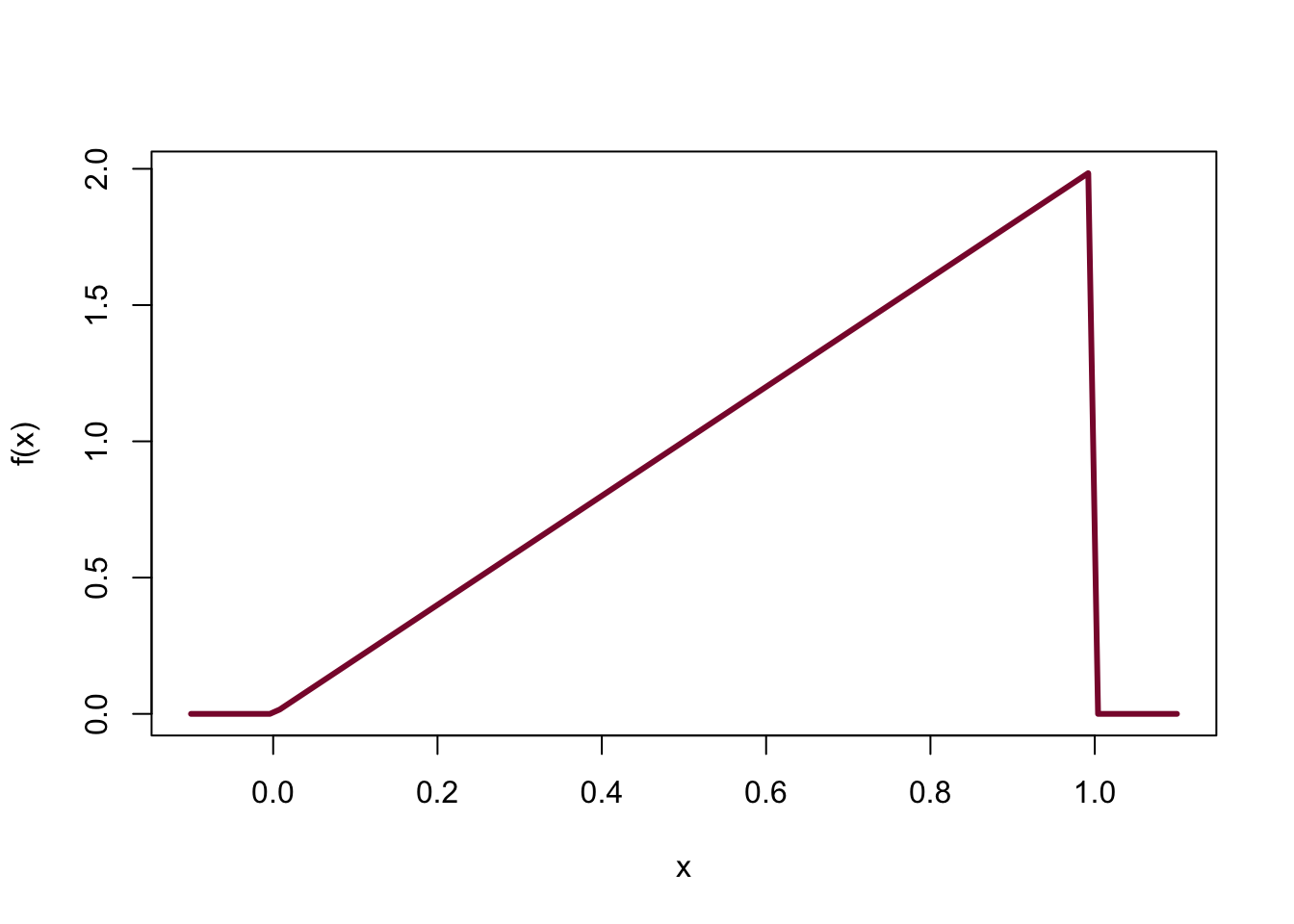
5.4 Cumulative distribution function
The cdf gives one language that works for discrete, continuous, and mixed variables.
The cumulative distribution function and survival function are
\[F_X(x)=\mathbb{P}(X\le x),\qquad S_X(x)=\mathbb{P}(X>x)=1-F_X(x).\]
Every cdf is nondecreasing, right-continuous, approaches 0 at \(-\infty\), and approaches 1 at \(+\infty\). Moreover,
\[\mathbb{P}(a<X\le b)=F_X(b)-F_X(a).\]
For a discrete variable, the jump at \(x\) equals \(\mathbb{P}(X=x)\). For a continuous variable, \(F_X'(x)=f_X(x)\) wherever the derivative exists. A mixed cdf has both jumps and smooth portions.
Example: a finite-support cdf
For a fair die \(W\), \(p_W(w)=1/6\) for \(w=1,\ldots,6\), and
\[ F_W(w)= \begin{cases} 0,&w<1,\\ k/6,&k\le w<k+1,\quad k=1,\ldots,5,\\ 1,&w\ge6. \end{cases} \]
The cdf is a step function whose jump at every support point equals \(1/6\).
Example: an infinite-support cdf
If \(T\) is the toss on which the first head appears, then
\[\mathbb{P}(T=t)=2^{-t},\qquad F_T(t)=1-2^{-t},\quad t=1,2,\ldots\]
The infinite-support cdf approaches 1 but never reaches it at a finite integer.
t <- 1:10
plot(t, 1 - 2^(-t), type = "s", ylim = c(0, 1),
     col = "#8A1538", lwd = 3, xlab = "t", ylab = "F(t)")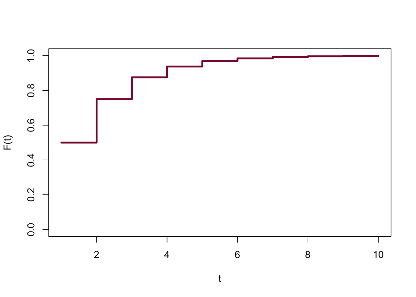
For example, the probability that the first head occurs on an even toss is
\[\mathbb{P}(T\text{ is even})=\sum_{j=1}^{\infty}2^{-2j}=\frac13.\]
Example: a continuous cdf on a finite interval
Let \(Y\) have density \(f_Y(y)=3y^2\) for \(0<y<1\). Integration gives
\[ F_Y(y)= \begin{cases} 0,&y<0,\\ y^3,&0\le y<1,\\ 1,&y\ge1. \end{cases} \]
Thus \(\mathbb{P}(Y\le1/2)=F_Y(1/2)=1/8\). The density describes the local concentration of probability; the cdf records all probability accumulated to the left.
Example: recovering a density from a cdf
Suppose
\[F_X(x)=\frac{1}{1+e^{-x}},\qquad -\infty<x<\infty.\]
Because this cdf is differentiable, its density is
\[f_X(x)=F_X'(x)=\frac{e^{-x}}{(1+e^{-x})^2}.\]
Example: integrating a piecewise density
Let
\[ f_X(x)= \begin{cases} 2x,&0<x<\tfrac12,\\ (4-2x)/3,&\tfrac12\le x<2,\\ 0,&\text{otherwise}. \end{cases} \]
When an interval crosses a point where the formula changes, split the integral there:
\[ \mathbb{P}(0.25<X\le1.25) =\int_{0.25}^{0.5}2x\,dx+\int_{0.5}^{1.25}\frac{4-2x}{3}\,dx =\frac34. \]
5.5 Mixed distributions
A mixed distribution combines probability masses at one or more points with a continuous density on one or more intervals.
For example, suppose \(Z\) equals 0 with probability \(1/2\) and has density \(f_Z(z)=z\) for \(0<z<1\). Then
\[\mathbb{P}(Z=0)+\int_0^1z\,dz=\frac12+\frac12=1.\]
The distinction between \(\mathbb{P}(0<Z<0.5)=0.125\) and \(\mathbb{P}(0\le Z<0.5)=0.625\) is the point mass at zero.
Its cdf makes the two components visible:
\[ F_Z(z)= \begin{cases} 0, & z<0,\\ \tfrac12, & z=0,\\ \tfrac12+\tfrac12z^2, & 0<z<1,\\ 1, & z\ge1. \end{cases} \]
The jump of size \(1/2\) at zero is the discrete mass; the smooth rise on \((0,1)\) is generated by the density.
Example: detecting a mixed distribution from its cdf
Consider \(F_X(x)=0\) for \(x<1\) and \(F_X(x)=1-e^{-x}\) for \(x\ge1\). At \(x=1\) the cdf jumps from 0 to \(1-e^{-1}\), so
\[\mathbb{P}(X=1)=1-e^{-1}.\]
For \(x>1\) the continuous component has density \(f_X(x)=e^{-x}\). A differentiable formula to the right of 1 does not erase the probability mass at the boundary.
5.6 Conditional distribution given an event
Probabilities often change after information becomes available. An insurer may study claim severity only among claims exceeding a deductible; a reliability engineer may update a lifetime model after a component has survived one year. We then need the entire updated distribution, not merely one conditional probability.
Let \(A\) be an event with \(\mathbb{P}(A)>0\). The conditional distribution of \(X\) given \(A\) has cdf
\[F_{X\mid A}(x)=\mathbb{P}(X\le x\mid A) =\frac{\mathbb{P}(\{X\le x\}\cap A)}{\mathbb{P}(A)}.\]
For a discrete variable,
\[p_{X\mid A}(x)=\frac{\mathbb{P}(\{X=x\}\cap A)}{\mathbb{P}(A)}.\]
When \(X\) is continuous and \(A\) restricts \(X\) to a region, the conditional density is
\[f_{X\mid A}(x)= \begin{cases} f_X(x)/\mathbb{P}(A),&x\text{ is compatible with }A,\\ 0,&\text{otherwise}. \end{cases}\]
Conditioning performs two operations: it removes values incompatible with the new information, then renormalizes the remaining masses or density so their total is again 1. The shape inside the retained region is proportional to the original shape.
Example: a truncated continuous distribution
Let \(f_X(x)=2x\) on \((0,1)\) and suppose we learn \(A=\{X\le1/2\}\). Since
\[\mathbb{P}(A)=\int_0^{1/2}2x\,dx=\frac14,\]
the conditional density is
\[ f_{X\mid A}(x)= \begin{cases} 8x,&0<x\le1/2,\\ 0,&\text{otherwise}. \end{cases} \]
It integrates to 1 on the shortened support. Its cdf is \(F_{X\mid A}(x)=4x^2\) for \(0\le x\le1/2\).
## 1 with absolute error < 1.1e-14curve(ifelse(x > 0 & x <= .5, 8*x, 0), 0, 1,
col = "#8A1538", lwd = 3,
xlab = "x", ylab = "Conditional density")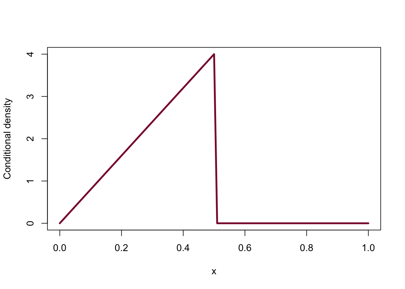
Example: conditioning a discrete waiting time
Let \(T\) be the toss of the first head, so \(p_T(t)=2^{-t}\) for \(t=1,2,\ldots\). Let \(A=\{T\text{ is odd}\}\). Then
\[\mathbb{P}(A)=\frac12+\frac1{2^3}+\frac1{2^5}+\cdots=\frac23,\]
and
\[ p_{T\mid A}(t)= \begin{cases} \dfrac32\,2^{-t},&t\text{ odd},\\ 0,&t\text{ even}. \end{cases} \]
Consequently,
\[\mathbb{P}(T\le3\mid T\text{ is odd}) =\frac{2^{-1}+2^{-3}}{2/3}=\frac{15}{16}=0.9375.\]
If instead \(B=\{T\le5\}\), then \(\mathbb{P}(B)=31/32\) and
\[\mathbb{P}(T\le3\mid T\le5)=\frac{7/8}{31/32}=\frac{28}{31}\approx0.9032.\]
t <- 1:15
p <- 2^(-t)
p_odd <- ifelse(t %% 2 == 1, p / (2/3), 0)
data.frame(toss = t, original_pmf = p,
           conditional_on_odd = p_odd)
## toss original_pmf conditional_on_odd
## 1 1 5.000000e-01 7.500000e-01
## 2 2 2.500000e-01 0.000000e+00
## 3 3 1.250000e-01 1.875000e-01
## 4 4 6.250000e-02 0.000000e+00
## 5 5 3.125000e-02 4.687500e-02
## 6 6 1.562500e-02 0.000000e+00
## 7 7 7.812500e-03 1.171875e-02
## 8 8 3.906250e-03 0.000000e+00
## 9 9 1.953125e-03 2.929688e-03
## 10 10 9.765625e-04 0.000000e+00
## 11 11 4.882812e-04 7.324219e-04
## 12 12 2.441406e-04 0.000000e+00
## 13 13 1.220703e-04 1.831055e-04
## 14 14 6.103516e-05 0.000000e+00
## 15 15 3.051758e-05 4.577637e-05## [1] 0.93755.7 Independent random variables
Random variables \(X\) and \(Y\) are independent if every event involving only \(X\) is independent of every event involving only \(Y\). Equivalently,
\[\mathbb{P}(X\in A,Y\in B)=\mathbb{P}(X\in A)\mathbb{P}(Y\in B)\]
for all appropriate sets \(A\) and \(B\).
Independence means that learning the value or range of one variable does not update the distribution of the other. Zero covariance alone does not generally imply independence.
Example: maximum of independent measurements
If \(X_1,\ldots,X_n\) are independent with common cdf \(F\), then
\[\mathbb{P}(\max_iX_i\le x)=\prod_{i=1}^n\mathbb{P}(X_i\le x)=[F(x)]^n.\]
The complement is often the simplest route to a maximum probability.
Similarly,
\[\mathbb{P}(\min_iX_i>x)=[1-F(x)]^n,\]
because the minimum exceeds \(x\) exactly when every observation exceeds \(x\).
Example: maximum and minimum densities
Let \(X_1,\ldots,X_4\) be independent with \(f(x)=2x\) on \((0,1)\), so \(F(x)=x^2\). For \(Y=\max_iX_i\),
\[F_Y(y)=[F(y)]^4=y^8,\qquad f_Y(y)=8y^7.\]
For \(Z=\min_iX_i\),
\[F_Z(z)=1-[1-z^2]^4,\qquad f_Z(z)=8z(1-z^2)^3.\]
The maximum is pushed toward 1, while the minimum is pushed toward 0.
Exercises
Exercise 1: identifying the model
Classify each variable as discrete, continuous, or mixed: annual claim count; exact claim severity; a policy payment that equals zero below a deductible and is continuous above it.
Show solution
Claim count is discrete; exact severity is continuous; the deductible payment is mixed because it has a mass at zero and a continuous positive part.Exercise 2: a pmf
Suppose \(p_X(x)=2/3^x\) for \(x=1,2,\ldots\). Verify that it is a pmf and find \(\mathbb{P}(X\text{ is even})\).
Show solution
The total is \(2\sum_{x=1}^{\infty}3^{-x}=1\). Thus
\[\mathbb{P}(X\text{ even})=2\sum_{j=1}^{\infty}3^{-2j}=\frac14.\]Exercise 3: recovering probability from a cdf
Let \(F(x)=0\) for \(x<0\), \(F(x)=x^2\) for \(0\le x<1\), and \(F(x)=1\) for \(x\ge1\). Find \(\mathbb{P}(0.25<X\le0.75)\) and the pdf.
Show solution
\[F(.75)-F(.25)=.75^2-.25^2=.5,\]
and \(f(x)=2x\) for \(0<x<1\), zero elsewhere.Exercise 4: independence and a maximum
Let \(X_1,X_2,X_3\) be independent with \(F(x)=x^3\) on \(0\le x\le1\). Find \(\mathbb{P}(\max X_i>1/2)\).
Show solution
\[1-[F(1/2)]^3=1-(1/8)^3=\frac{511}{512}.\]Exercise 5: conditional distribution
Let \(X\) have density \(f(x)=e^{-x}\) for \(x>0\). Find the conditional density of \(X\) given \(X>1\), and calculate \(\mathbb{P}(X\le2\mid X>1)\).
Show solution
Since \(\mathbb{P}(X>1)=e^{-1}\),
\[f_{X\mid X>1}(x)=\frac{e^{-x}}{e^{-1}}=e^{-(x-1)},\qquad x>1,\]
and it is zero otherwise. Therefore
\[\mathbb{P}(X\le2\mid X>1)=\int_1^2e^{-(x-1)}\,dx=1-e^{-1}.\]Exercise 6: a mixed cdf
Suppose \(F(x)=0\) for \(x<1\) and \(F(x)=1-e^{-x}\) for \(x\ge1\). Find \(\mathbb{P}(X=1)\) and \(\mathbb{P}(1<X\le2)\).
Show solution
The jump at 1 is
\[\mathbb{P}(X=1)=F(1)-F(1^-)=1-e^{-1}.\]
The continuous probability to the right is
\[\mathbb{P}(1<X\le2)=F(2)-F(1)=e^{-1}-e^{-2}.\]5.8 Chapter summary
A random variable maps experimental outcomes to numbers. Discrete distributions use masses, continuous distributions use areas, and mixed distributions use both. The cdf unifies all three types. Conditioning restricts and renormalizes a distribution after new information, while independence permits joint probabilities to factor into products.