Chapter 9 Bivariate Random Variables
9.1 Learning goals
Many real problems involve quantities that must be studied together: price and demand, claim frequency and claim severity, rainfall and crop yield, or the returns of two investments. A bivariate model preserves information about each variable and about how the two variables move together.
After this chapter, you should be able to:
- construct and interpret joint, marginal, and conditional distributions;
- compute expectations of functions of two random variables;
- calculate and interpret covariance and correlation;
- find variances and covariances of linear combinations;
- recognize and use a bivariate Normal model;
- distinguish independence from absence of correlation;
- compute conditional means and variances and apply the laws of total expectation and total variance.
9.2 Joint distributions
A separate model for \(X\) and another for \(Y\) is not enough to answer questions such as “How likely are large values of both variables?” Two pairs can have identical marginal distributions but completely different dependence. The joint distribution supplies the missing information.
A bivariate random vector \((X,Y)\) assigns a pair of real numbers to every outcome of a random experiment. Its joint cumulative distribution function is
\[ F_{X,Y}(x,y)=\mathbb{P}(X\leq x,\,Y\leq y). \]
It describes the probability accumulated in the region to the lower left of \((x,y)\).
9.2.1 Discrete joint distributions
If \(X\) and \(Y\) are discrete, their joint probability mass function is
\[ p_{X,Y}(x,y)=\mathbb{P}(X=x,Y=y). \]
It must satisfy
\[ p_{X,Y}(x,y)\geq0 \quad\text{and}\quad \sum_x\sum_y p_{X,Y}(x,y)=1. \]
Probabilities of events are found by adding the masses of all pairs in the event:
\[ \mathbb{P}\big((X,Y)\in A\big) =\sum_{(x,y)\in A}p_{X,Y}(x,y). \]
Example: insurance claim indicators
Let \(X\) indicate whether an automobile policy produces a collision claim and let \(Y\) indicate whether it produces a glass claim during the same year. Suppose their joint pmf is shown below. The first column identifies the value of the collision-claim indicator; the next two columns identify the value of the glass-claim indicator.
| Collision claim, X | No glass claim, Y = 0 | Glass claim, Y = 1 | Row total |
|---|---|---|---|
| No collision claim, X = 0 | 0.90 | 0.04 | 0.94 |
| Collision claim, X = 1 | 0.05 | 0.01 | 0.06 |
| Column total | 0.95 | 0.05 | 1.00 |
The probability of at least one type of claim is
\[ \mathbb{P}(X=1\text{ or }Y=1)=0.05+0.01+0.04=0.10. \]
The entry \(0.01\) is not merely another probability: it measures how often the two claim types occur together. That co-occurrence will later influence covariance and aggregate risk.
9.2.2 Continuous joint distributions
If \(X\) and \(Y\) are continuous, a joint probability density function satisfies
\[ f_{X,Y}(x,y)\geq0, \qquad \int_{-\infty}^{\infty}\int_{-\infty}^{\infty} f_{X,Y}(x,y)\,dy\,dx=1. \]
For a region \(A\) in the plane,
\[ \mathbb{P}\big((X,Y)\in A\big) =\iint_A f_{X,Y}(x,y)\,dA. \]
The density is a surface; probability is volume beneath that surface over a region. As in the univariate continuous case, \(f_{X,Y}(x,y)\) is not a point probability and \(\mathbb{P}(X=x,Y=y)=0\).
Example: probability over a triangular support
Suppose
\[ f_{X,Y}(x,y)=2, \qquad 0<y<x<1, \]
and the density is zero elsewhere. The support is triangular, so the integration limits must reflect \(0<y<x<1\). Its total probability is
\[ \int_0^1\int_0^x2\,dy\,dx =\int_0^1 2x\,dx=1. \]
For example,
\[ \mathbb{P}(X\leq 0.6,\,Y\leq0.3) =\int_0^{0.3}\int_y^{0.6}2\,dx\,dy =0.27. \]
The limits are the main intellectual step: for each fixed \(y\), the condition \(y<x\leq0.6\) determines the allowed values of \(x\).
Exercise: checking a joint pmf
A proposed joint pmf has support \(x,y\in\{0,1\}\) and values proportional to \(x+y+1\). Find the constant of proportionality and compute \(\mathbb{P}(X=Y)\).
Show solution
Write \(p(x,y)=c(x+y+1)\). The four weights are \(1,2,2,3\), whose sum is \(8\), so \(c=1/8\). Therefore
\[ \mathbb{P}(X=Y)=p(0,0)+p(1,1)=\frac18+\frac38=\frac12. \]
Exercise: integrating over a region
Let \(f_{X,Y}(x,y)=2\) on \(0<y<x<1\). Find \(\mathbb{P}(X+Y<1)\).
Show solution
Both \(y<x\) and \(y<1-x\) must hold. The upper boundary changes where \(x=1-x\), namely at \(x=1/2\):
\[ \begin{aligned} \mathbb{P}(X+Y<1) &=\int_0^{1/2}\int_0^x2\,dy\,dx +\int_{1/2}^1\int_0^{1-x}2\,dy\,dx\\ &=\frac14+\frac14=\frac12. \end{aligned} \]
9.3 Marginal distributions
Sometimes the pair is modeled jointly, but the question concerns only one component. We then “ignore” the other variable by accumulating its probability over every possible value.
The marginal distributions are obtained from the joint distribution by summing or integrating out the other variable.
For discrete variables,
\[ p_X(x)=\sum_y p_{X,Y}(x,y), \qquad p_Y(y)=\sum_x p_{X,Y}(x,y). \]
For continuous variables,
\[ f_X(x)=\int_{-\infty}^{\infty}f_{X,Y}(x,y)\,dy, \qquad f_Y(y)=\int_{-\infty}^{\infty}f_{X,Y}(x,y)\,dx. \]
“Marginal” comes from displaying row and column totals in the margins of a joint probability table.
Example: marginals from a discrete table
Consider the following joint table. Its interior cells contain the joint pmf, while the final row and column contain the marginal pmfs.
| Value of X | Y = 0 | Y = 1 | Marginal probability of X |
|---|---|---|---|
| X = 0 | 0.30 | 0.20 | 0.50 |
| X = 1 | 0.10 | 0.40 | 0.50 |
| Marginal probability of Y | 0.40 | 0.60 | 1.00 |
Adding across rows gives \(p_X(0)=p_X(1)=0.5\); adding down columns gives \(p_Y(0)=0.4\) and \(p_Y(1)=0.6\). The marginals describe each variable separately, but the four interior cells are still needed to describe their association.
Example: marginals from a triangular density
For \(f_{X,Y}(x,y)=2\) on \(0<y<x<1\),
\[ f_X(x)=\int_0^x2\,dy=2x, \qquad 0<x<1, \]
whereas
\[ f_Y(y)=\int_y^1 2\,dx=2(1-y), \qquad 0<y<1. \]
The two marginals have different shapes even though they arise from the same joint density. The support explains why: \(Y<X\) always.
Exercise: finding continuous marginals
Suppose \(f_{X,Y}(x,y)=x+y\) on the unit square \(0<x<1\), \(0<y<1\). Verify that this is a density and find \(f_X\) and \(f_Y\).
Show solution
The density is nonnegative and
\[ \int_0^1\int_0^1(x+y)\,dy\,dx=\frac12+\frac12=1. \]
Thus
\[ f_X(x)=\int_0^1(x+y)\,dy=x+\frac12, \quad f_Y(y)=\int_0^1(x+y)\,dx=y+\frac12, \]
on \((0,1)\), and both are zero elsewhere.
9.4 Expectation of bivariate random variables
Expectation converts a joint distribution into useful summaries. We may want the average of one component, a product such as \(XY\), a total \(X+Y\), or a nonlinear cost \(g(X,Y)\).
For any function \(g\) for which the expectation exists,
\[ \mathbb{E}\{g(X,Y)\} =\sum_x\sum_y g(x,y)p_{X,Y}(x,y) \]
in the discrete case, and
\[ \mathbb{E}\{g(X,Y)\} =\int_{-\infty}^{\infty}\int_{-\infty}^{\infty} g(x,y)f_{X,Y}(x,y)\,dy\,dx \]
in the continuous case.
Linearity does not require independence:
\[ \mathbb{E}(aX+bY+c) =a\mathbb{E}(X)+b\mathbb{E}(Y)+c. \]
Example: expected joint cost for discrete risks
Use the discrete table with probabilities \(0.30,0.20,0.10,0.40\). Suppose the cost is
\[ g(X,Y)=100X+60Y+40XY. \]
The interaction term adds a coordination cost when both events occur. From the table,
\[ \mathbb{E}(X)=0.5, \quad \mathbb{E}(Y)=0.6, \quad \mathbb{E}(XY)=0.4. \]
Therefore
\[ \mathbb{E}\{g(X,Y)\} =100(0.5)+60(0.6)+40(0.4)=102. \]
Example: a continuous expectation
For the triangular density \(f_{X,Y}(x,y)=2\) on \(0<y<x<1\),
\[ \mathbb{E}(X) =\int_0^1\int_0^x2x\,dy\,dx =\frac23, \]
\[ \mathbb{E}(Y) =\int_0^1\int_0^x2y\,dy\,dx =\frac13, \]
and
\[ \mathbb{E}(XY) =\int_0^1\int_0^x2xy\,dy\,dx =\frac14. \]
The inequalities built into the support are visible in the means: because \(Y<X\) with probability one, it is natural that \(\mathbb{E}(Y)<\mathbb{E}(X)\).
9.5 Covariance and correlation
Marginal means and variances say nothing about whether two variables tend to be high or low together. Covariance records the direction of their linear co-movement, and correlation removes the effect of measurement units.
Provided the relevant moments exist, the covariance is
\[ \operatorname{Cov}(X,Y) =\mathbb{E}\!\left[(X-\mathbb{E}X)(Y-\mathbb{E}Y)\right] =\mathbb{E}(XY)-\mathbb{E}(X)\mathbb{E}(Y). \]
If both standard deviations are positive, the correlation is
\[ \rho_{X,Y}=\operatorname{Corr}(X,Y) =\frac{\operatorname{Cov}(X,Y)} {\sqrt{\operatorname{Var}(X)}\sqrt{\operatorname{Var}(Y)}}. \]
A positive covariance means values above their respective means tend to occur together. A negative covariance means a value above its mean tends to accompany the other below its mean. Correlation is unit-free and lies in \([-1,1]\), but it measures linear association only.
Example: covariance from a joint table
For the discrete table,
\[ \mathbb{E}(X)=0.5, \quad \mathbb{E}(Y)=0.6, \quad \mathbb{E}(XY)=0.4. \]
Thus
\[ \operatorname{Cov}(X,Y)=0.4-(0.5)(0.6)=0.1. \]
Because \(X\) and \(Y\) are indicators, \(\operatorname{Var}(X)=0.5(0.5)=0.25\) and \(\operatorname{Var}(Y)=0.6(0.4)=0.24\). Hence
\[ \rho_{X,Y} =\frac{0.1}{\sqrt{0.25(0.24)}} \approx0.408. \]
The association is positive but not perfect.
Example: covariance for a continuous pair
For the triangular density,
\[ \operatorname{Cov}(X,Y) =\frac14-\left(\frac23\right)\left(\frac13\right) =\frac1{36}>0. \]
Although the support requires \(Y<X\), large values of \(X\) leave more room for large values of \(Y\), producing positive association.
Exercise: interpreting a change of units
Suppose \(C=100X\) converts an amount from hundreds of riyals to riyals and \(D=60Y\) converts minutes to seconds. Express \(\operatorname{Cov}(C,D)\) and \(\operatorname{Corr}(C,D)\) in terms of the corresponding quantities for \(X\) and \(Y\).
Show solution
\[ \operatorname{Cov}(C,D)=100(60)\operatorname{Cov}(X,Y) =6000\operatorname{Cov}(X,Y). \]
Positive changes of units do not alter correlation, so
\[ \operatorname{Corr}(C,D)=\operatorname{Corr}(X,Y). \]
9.6 Variance and covariance of sums
Totals are central in applications: a portfolio return is a weighted sum of asset returns, an insurer’s aggregate loss is a sum of claim amounts, and a measurement may combine several noisy components. Dependence determines how the risks combine.
For constants \(a,b\),
\[ \operatorname{Var}(aX+bY) =a^2\operatorname{Var}(X)+b^2\operatorname{Var}(Y) +2ab\operatorname{Cov}(X,Y). \]
More generally,
\[ \operatorname{Var}\!\left(\sum_{i=1}^n a_iX_i\right) =\sum_{i=1}^n a_i^2\operatorname{Var}(X_i) +2\sum_{i<j}a_i a_j\operatorname{Cov}(X_i,X_j). \]
If the variables are pairwise uncorrelated, all cross-covariance terms vanish.
Covariance is bilinear. In particular,
\[ \operatorname{Cov}(aX+bY,cU+dV) =ac\operatorname{Cov}(X,U)+ad\operatorname{Cov}(X,V) +bc\operatorname{Cov}(Y,U)+bd\operatorname{Cov}(Y,V). \]
Consequently,
\[ \operatorname{Cov}\!\left(\sum_i a_iX_i,\sum_j b_jY_j\right) =\sum_i\sum_j a_i b_j\operatorname{Cov}(X_i,Y_j). \]
Example: portfolio variance and diversification
Let two asset returns have
\[ \sigma_1=0.18, \qquad \sigma_2=0.12, \qquad \rho=0.25. \]
A portfolio invests \(60\%\) in the first asset and \(40\%\) in the second, so \(R_P=0.6R_1+0.4R_2\). Since
\[ \operatorname{Cov}(R_1,R_2)=\rho\sigma_1\sigma_2 =0.25(0.18)(0.12)=0.0054, \]
the portfolio variance is
\[ \begin{aligned} \operatorname{Var}(R_P) &=(0.6)^2(0.18)^2+(0.4)^2(0.12)^2\\ &\quad+2(0.6)(0.4)(0.0054)\\ &=0.01656. \end{aligned} \]
Thus \(\operatorname{sd}(R_P)\approx0.1287\). The weighted average of the two standard deviations is \(0.156\), which is larger. Imperfect correlation creates the diversification benefit; it does not come merely from owning two assets.
Example: aggregate insurance loss
Let \(X_i\) be the loss from policy \(i\), with \(\operatorname{Var}(X_i)=400\) for each of \(100\) policies. Suppose every distinct pair has covariance \(2\) because all policies share a small weather exposure. For \(S=\sum_{i=1}^{100}X_i\),
\[ \begin{aligned} \operatorname{Var}(S) &=100(400)+2\binom{100}{2}(2)\\ &=59{,}800. \end{aligned} \]
If the policies had been independent, the variance would have been only \(40{,}000\). Small pairwise covariances can accumulate across many pairs, which is why common shocks matter greatly in insurance portfolios.
Example: covariance of two totals
Let quarterly sales be \(S=X_1+X_2\) and advertising expenditure be \(A=Y_1+Y_2\). Then
\[ \operatorname{Cov}(S,A) =\operatorname{Cov}(X_1,Y_1)+\operatorname{Cov}(X_1,Y_2) +\operatorname{Cov}(X_2,Y_1)+\operatorname{Cov}(X_2,Y_2). \]
This expansion forces us to include both same-period and cross-period relationships. Ignoring the latter is justified only when the model says they are zero.
Exercise: variance of a difference
Suppose \(\operatorname{Var}(X)=9\), \(\operatorname{Var}(Y)=4\), and \(\operatorname{Cov}(X,Y)=3\). Find \(\operatorname{Var}(2X-Y)\) and explain the sign of the covariance term.
Show solution
\[ \operatorname{Var}(2X-Y) =4(9)+1(4)+2(2)(-1)(3)=28. \]
The covariance term is negative because the coefficients of \(X\) and \(Y\) have opposite signs. Positive co-movement makes the difference less variable.
9.7 The bivariate Normal distribution
The bivariate Normal model is a particularly useful example because its entire dependence structure is determined by means, variances, and correlation, and because every linear combination remains Normal.
The vector \((X,Y)\) has a bivariate Normal distribution with means \(\mu_X,\mu_Y\), standard deviations \(\sigma_X,\sigma_Y\), and correlation \(\rho\) if its joint density is
\[ \begin{aligned} f_{X,Y}(x,y) &=\frac{1}{2\pi\sigma_X\sigma_Y\sqrt{1-\rho^2}}\\ &\quad\times\exp\!\left[-\frac{1}{2(1-\rho^2)} \left\{ \left(\frac{x-\mu_X}{\sigma_X}\right)^2 -2\rho\left(\frac{x-\mu_X}{\sigma_X}\right) \left(\frac{y-\mu_Y}{\sigma_Y}\right) +\left(\frac{y-\mu_Y}{\sigma_Y}\right)^2 \right\}\right], \end{aligned} \]
for \(-1<\rho<1\).
Its marginal distributions are Normal, and
\[ aX+bY\sim N\!\left( a\mu_X+b\mu_Y, a^2\sigma_X^2+b^2\sigma_Y^2+2ab\rho\sigma_X\sigma_Y \right). \]
Example: a Normal portfolio return
Suppose \((R_1,R_2)\) is bivariate Normal with means \(0.06\) and \(0.04\), standard deviations \(0.15\) and \(0.10\), and correlation \(0.30\). For \(R_P=0.7R_1+0.3R_2\),
\[ \mathbb{E}(R_P)=0.7(0.06)+0.3(0.04)=0.054, \]
and
\[ \operatorname{Var}(R_P) =(0.7)^2(0.15)^2+(0.3)^2(0.10)^2 +2(0.7)(0.3)(0.30)(0.15)(0.10) =0.013815. \]
Therefore \(R_P\sim N(0.054,0.013815)\). Here the Normal assumption supplies more than the first two moments: it gives the full distribution of the portfolio return.
9.7.1 Interactive bivariate Normal explorer
Change the means, standard deviations, and correlation. The burgundy points form a reproducible simulated sample; the gold ellipses are equal-density contours. Correlation controls the direction and elongation of the contours, while the marginal standard deviations control their spread.
Exercise: a linear combination of bivariate Normals
Let \((X,Y)\) be bivariate Normal with \(\mu_X=10\), \(\mu_Y=4\), \(\sigma_X=3\), \(\sigma_Y=2\), and \(\rho=-0.5\). Find the distribution of \(T=X+2Y\).
Show solution
The mean is \(10+2(4)=18\). Also,
\[ \operatorname{Var}(T) =3^2+2^2(2^2)+2(1)(2)(-0.5)(3)(2) =9+16-12=13. \]
Thus \(T\sim N(18,13)\), where the second parameter denotes the variance.
9.8 Independence
Knowing the marginals usually does not determine the joint distribution. Independence is the special case in which the marginals do determine it completely.
Random variables \(X\) and \(Y\) are independent if
\[ F_{X,Y}(x,y)=F_X(x)F_Y(y) \]
for all \(x,y\). Equivalently, wherever the pmfs or densities exist,
\[ p_{X,Y}(x,y)=p_X(x)p_Y(y) \]
in the discrete case, or
\[ f_{X,Y}(x,y)=f_X(x)f_Y(y) \]
in the continuous case.
If \(X\) and \(Y\) are independent and the expectations exist, then
\[ \mathbb{E}\{g(X)h(Y)\} =\mathbb{E}\{g(X)\}\mathbb{E}\{h(Y)\}. \]
Example: testing independence in a table
In the discrete table, \(p_{X,Y}(1,1)=0.40\), while
\[ p_X(1)p_Y(1)=(0.50)(0.60)=0.30. \]
Because even one pair violates the factorization, \(X\) and \(Y\) are not independent.
Example: factorization of a continuous density
Suppose
\[ f_{X,Y}(x,y)=4xy, \qquad 0<x<1,\;0<y<1. \]
The marginals are \(f_X(x)=2x\) and \(f_Y(y)=2y\). Since
\[ f_{X,Y}(x,y)=(2x)(2y)=f_X(x)f_Y(y) \]
on a rectangular support, \(X\) and \(Y\) are independent.
Remark — independence versus uncorrelatedness. If \(X\) and \(Y\) are independent and have finite second moments, then
\[ \operatorname{Cov}(X,Y)=0. \]
Thus, independence always implies uncorrelatedness when the covariance exists. The converse is generally false: zero covariance only says that there is no linear association; it does not rule out a nonlinear relationship.
For example, let \(X\) be equally likely to be \(-1,0,\) or \(1\), and set \(Y=X^2\). Then \(Y\) is completely determined by \(X\), so they are dependent. Yet
\[ \operatorname{Cov}(X,Y) =\mathbb{E}(X^3)-\mathbb{E}(X)\mathbb{E}(X^2)=0. \]
The converse becomes true under an important additional assumption: if \((X,Y)\) has a jointly bivariate Normal distribution, then
\[ \operatorname{Cov}(X,Y)=0 \quad\Longleftrightarrow\quad X\text{ and }Y\text{ are independent}. \]
Indeed, the bivariate Normal density contains dependence through the correlation parameter \(\rho\). When the marginal variances are positive, \(\operatorname{Cov}(X,Y)=0\) is equivalent to \(\rho=0\); the joint density then factorizes as \(f_{X,Y}(x,y)=f_X(x)f_Y(y)\). The conclusion also remains valid for a possibly degenerate jointly Gaussian pair, although one or both variables may then be constant. This equivalence is special to the jointly Normal family and must not be assumed for arbitrary distributions.
Exercise: independence or not?
Suppose \(p_{X,Y}(x,y)=c(x+1)(y+1)\) for \(x,y\in\{0,1\}\). Find \(c\) and determine whether \(X\) and \(Y\) are independent.
Show solution
The sum of \((x+1)(y+1)\) over the four pairs is \((1+2)(1+2)=9\), so \(c=1/9\). The marginals are
\[ p_X(x)=\frac{x+1}{3}, \qquad p_Y(y)=\frac{y+1}{3}. \]
Their product is \((x+1)(y+1)/9=p_{X,Y}(x,y)\), so the variables are independent.
9.9 Conditional distributions
New information restricts the possible outcomes and redistributes probability over what remains. A conditional distribution is therefore an updated distribution, not merely a single conditional probability.
For discrete variables with \(p_Y(y)>0\), the conditional pmf of \(X\) given \(Y=y\) is
\[ p_{X\mid Y}(x\mid y) =\frac{p_{X,Y}(x,y)}{p_Y(y)}. \]
For continuous variables with \(f_Y(y)>0\), the conditional density is
\[ f_{X\mid Y}(x\mid y) =\frac{f_{X,Y}(x,y)}{f_Y(y)}. \]
Conditioning selects a row, column, or slice of the joint distribution and then rescales it so that its total probability becomes one.
Example: a discrete conditional distribution
For the discrete table,
\[ \mathbb{P}(X=0\mid Y=1)=\frac{0.20}{0.60}=\frac13, \qquad \mathbb{P}(X=1\mid Y=1)=\frac{0.40}{0.60}=\frac23. \]
Before observing \(Y\), \(\mathbb{P}(X=1)=0.5\). Observing \(Y=1\) raises it to \(2/3\), which is another way to see the positive association.
Example: a continuous conditional density
For \(f_{X,Y}(x,y)=2\) on \(0<y<x<1\), the marginal density is \(f_Y(y)=2(1-y)\). Therefore, for fixed \(0<y<1\),
\[ f_{X\mid Y}(x\mid y) =\frac{2}{2(1-y)} =\frac{1}{1-y}, \qquad y<x<1. \]
Thus, after observing \(Y=y\), \(X\) is uniform on \((y,1)\). The observation changes both the support and the density.
9.9.1 Conditional distribution given an event
We often condition on an event rather than an exact value, such as “the loss exceeded the deductible” or “the first head occurred on an odd toss.”
If \(A\) is an event with \(\mathbb{P}(A)>0\), the conditional distribution of \(X\) given \(A\) is defined by
\[ \mathbb{P}(X\in B\mid A) =\frac{\mathbb{P}(\{X\in B\}\cap A)}{\mathbb{P}(A)}. \]
For a discrete \(X\),
\[ p_{X\mid A}(x)=\frac{\mathbb{P}(X=x,A)}{\mathbb{P}(A)}. \]
If \(A\) is determined by \(X\) itself, the original pmf or density is restricted to the values allowed by \(A\) and then renormalized.
Example: conditioning a discrete waiting time
Let \(X\) be the toss on which the first head appears for a fair coin, so \(\mathbb{P}(X=x)=2^{-x}\) for \(x=1,2,\ldots\). Let \(A\) be the event that \(X\) is odd. Then
\[ \mathbb{P}(A)=\frac12+\frac1{2^3}+\frac1{2^5}+\cdots=\frac23. \]
Consequently,
\[ p_{X\mid A}(x)= \begin{cases} \dfrac{3}{2^{x+1}}, & x\text{ odd},\\ 0, & x\text{ even}. \end{cases} \]
The conditional distribution removes every even value and rescales the remaining probabilities.
Example: conditioning a continuous loss
Suppose \(X\) has density \(f_X(x)=2x\) for \(0<x<1\), and let \(A=\{X\leq1/2\}\). Since
\[ \mathbb{P}(A)=\int_0^{1/2}2x\,dx=\frac14, \]
the conditional density is
\[ f_{X\mid A}(x)= \begin{cases} 8x, & 0<x\leq1/2,\\ 0, & \text{otherwise}. \end{cases} \]
The factor \(4\) is the renormalization needed after retaining only one quarter of the original probability.
Exercise: a conditional pmf
For the discrete table, find the conditional distribution of \(Y\) given \(X=0\) and compute \(\mathbb{P}(Y=1\mid X=0)\).
Show solution
The row total is \(p_X(0)=0.50\). Therefore
\[ p_{Y\mid X}(0\mid0)=\frac{0.30}{0.50}=0.60, \qquad p_{Y\mid X}(1\mid0)=\frac{0.20}{0.50}=0.40. \]
Thus \(\mathbb{P}(Y=1\mid X=0)=0.40\).
9.10 Conditional mean and conditional variance
A conditional distribution can be summarized just like an ordinary distribution. Its mean is the best mean-square prediction after the conditioning information is known; its variance measures the uncertainty that remains.
For discrete variables,
\[ \mathbb{E}(X\mid Y=y) =\sum_x x\,p_{X\mid Y}(x\mid y), \]
and for continuous variables,
\[ \mathbb{E}(X\mid Y=y) =\int_{-\infty}^{\infty}x f_{X\mid Y}(x\mid y)\,dx. \]
The conditional variance is
\[ \operatorname{Var}(X\mid Y=y) =\mathbb{E}(X^2\mid Y=y) -\{\mathbb{E}(X\mid Y=y)\}^2. \]
As \(y\) varies, \(\mathbb{E}(X\mid Y=y)\) is itself a function of the random variable \(Y\), written \(\mathbb{E}(X\mid Y)\).
Example: conditional moments in the discrete case
For the table, \(X\) is an indicator. Given \(Y=1\), its conditional success probability is \(2/3\). Hence
\[ \mathbb{E}(X\mid Y=1)=\frac23, \qquad \operatorname{Var}(X\mid Y=1) =\frac23\left(1-\frac23\right)=\frac29. \]
Given \(Y=0\), the corresponding probability is \(0.10/0.40=1/4\), so
\[ \mathbb{E}(X\mid Y=0)=\frac14, \qquad \operatorname{Var}(X\mid Y=0)=\frac3{16}. \]
Example: conditional moments in the continuous case
For the triangular model, \(X\mid Y=y\) is uniform on \((y,1)\). Therefore
\[ \mathbb{E}(X\mid Y=y)=\frac{y+1}{2}, \qquad \operatorname{Var}(X\mid Y=y)=\frac{(1-y)^2}{12}. \]
As \(y\) increases, the conditional mean rises while the conditional variance falls: knowing that \(Y\) is close to one forces \(X\) into a short interval just above \(Y\).
The law of total expectation is
\[ \mathbb{E}(X)=\mathbb{E}\{\mathbb{E}(X\mid Y)\}. \]
The law of total variance is
\[ \operatorname{Var}(X) =\mathbb{E}\{\operatorname{Var}(X\mid Y)\} +\operatorname{Var}\{\mathbb{E}(X\mid Y)\}. \]
Total variance separates uncertainty into two parts: average uncertainty within groups defined by \(Y\), and variability between their conditional means. This decomposition is fundamental in hierarchical models, credibility theory, random-effects models, and analysis of variance.
Example: decomposing claim variability
Suppose a policyholder is low-risk with probability \(0.8\) and high-risk with probability \(0.2\). Let \(X\) be an annual claim indicator with
\[ \mathbb{P}(X=1\mid Y=L)=0.05, \qquad \mathbb{P}(X=1\mid Y=H)=0.30. \]
The law of total expectation gives
\[ \mathbb{E}(X)=0.8(0.05)+0.2(0.30)=0.10. \]
For total variance,
\[ \mathbb{E}\{\operatorname{Var}(X\mid Y)\} =0.8(0.05)(0.95)+0.2(0.30)(0.70)=0.08, \]
and
\[ \operatorname{Var}\{\mathbb{E}(X\mid Y)\} =0.8(0.05-0.10)^2+0.2(0.30-0.10)^2=0.01. \]
Thus \(\operatorname{Var}(X)=0.09\), which agrees with the variance of a Bernoulli variable having marginal probability \(0.10\).
Exercise: conditional mean and total expectation
Let \(Y\) take values \(0\) and \(1\) with equal probability. Given \(Y=y\), suppose \(X\) has mean \(2+y\) and variance \(1+2y\). Find \(\mathbb{E}(X)\) and \(\operatorname{Var}(X)\).
Show solution
\[ \mathbb{E}(X)=\frac12(2)+\frac12(3)=\frac52. \]
Also,
\[ \mathbb{E}\{\operatorname{Var}(X\mid Y)\} =\frac12(1)+\frac12(3)=2, \]
while \(\mathbb{E}(X\mid Y)\) is equally likely to be \(2\) or \(3\), so its variance is \(1/4\). Hence
\[ \operatorname{Var}(X)=2+\frac14=\frac94. \]
Exercise: conditional moments from a density
For \(f_{X,Y}(x,y)=4xy\) on the unit square, find \(\mathbb{E}(X\mid Y=y)\) and \(\operatorname{Var}(X\mid Y=y)\).
Show solution
Because \(f_{X,Y}(x,y)=f_X(x)f_Y(y)\), the variables are independent. Thus the conditional distribution of \(X\) is its marginal density \(f_X(x)=2x\), \(0<x<1\). Therefore
\[ \mathbb{E}(X\mid Y=y)=\int_0^1x(2x)\,dx=\frac23, \]
and
\[ \operatorname{Var}(X\mid Y=y) =\int_0^1x^2(2x)\,dx-\left(\frac23\right)^2 =\frac12-\frac49=\frac1{18}. \]
Neither quantity depends on \(y\), as independence suggests.
9.11 Case study: Ozone and temperature in New York
9.11.1 Purpose and context
The real airquality dataset contains daily New York air-quality measurements from May through September 1973. The purpose is to study a joint distribution, derive marginal and conditional summaries, quantify dependence, and evaluate whether a bivariate Normal description is plausible for ozone and temperature.
Let \(X\) be ozone concentration and \(Y\) be temperature for complete observation days.
9.11.2 Guided questions
- How many complete records are available? Describe the marginal distributions of \(X\) and \(Y\).
- Draw the joint scatterplot and interpret its direction, form, and strength.
- Compute \(\mathbb{E}(X)\), \(\mathbb{E}(Y)\), \(\mathrm{Cov}(X,Y)\), and \(\mathrm{Corr}(X,Y)\).
- Estimate \(\mathbb{E}(X\mid Y\geq80)\) and \(\mathbb{E}(X\mid Y<80)\). What changes after conditioning?
- Are ozone and temperature plausibly independent? Give graphical and numerical evidence.
- Standardize both variables and identify observations outside a 95% bivariate Normal ellipse using Mahalanobis distance.
- Simulate from a fitted bivariate Normal model and compare its scatterplot with the real data.
- Define a standardized environmental index \(I=0.6Z_X+0.4Z_Y\). Compute its variance from the covariance formula and verify it empirically.
- What limitations arise from missing data, seasonality, nonlinearity, and the Normal assumption?
Show solution and R analysis
There are 116 complete records. Ozone has mean \(42.13\), median \(31.50\), and standard deviation \(32.99\) ppb; its large upper tail (maximum \(168\)) makes it distinctly right-skewed. Temperature has mean \(77.87\), median \(79\), and standard deviation \(9.49^{\circ}\)F and is much closer to a symmetric distribution.
The scatterplot has a clear positive direction and moderately strong association, although its changing spread and a few high-ozone observations depart from a perfectly elliptical cloud. Numerically,
\[ \mathbb{E}(X)\approx42.13, \qquad \mathbb{E}(Y)\approx77.87, \]
\[ \mathrm{Cov}(X,Y)\approx218.52, \qquad \mathrm{Corr}(X,Y)\approx0.698. \]
Conditioning changes the ozone distribution substantially:
\[ \mathbb{E}(X\mid Y\geq80)\approx62.39, \qquad \mathbb{E}(X\mid Y<80)\approx22.56. \]
The scatterplot and correlation provide strong evidence against independence: warmer days tend to have much higher ozone. They do not, however, establish that temperature alone causes ozone changes.
For standardized observations \(Z=(Z_X,Z_Y)^\mathsf{T}\), the squared Mahalanobis distance is
\[ D^2=Z^\mathsf{T}R^{-1}Z, \]
where \(R\) is the sample correlation matrix. Comparing \(D^2\) with the 95th percentile of a \(\chi^2_2\) distribution identifies four observations outside the fitted 95% ellipse: original dataset rows 30, 62, 99, and 117. Their ozone values are unusually high relative to temperature.
A fitted bivariate Normal simulation reproduces the positive elliptical tendency, but not the pronounced ozone skewness, tail behavior, or every feature of the real cloud. Thus it is a useful approximation, not a complete model.
Because \(Z_X\) and \(Z_Y\) each have variance 1,
\[ \begin{aligned} \mathrm{Var}(I) &=0.6^2+0.4^2+2(0.6)(0.4)\mathrm{Corr}(X,Y)\\ &\approx0.8552. \end{aligned} \]
The empirical variance of the computed index is also \(0.8552\), confirming the covariance formula.
## [1] 116## Ozone Temp
## Min. : 1.00 Min. :57.00
## 1st Qu.: 18.00 1st Qu.:71.00
## Median : 31.50 Median :79.00
## Mean : 42.13 Mean :77.87
## 3rd Qu.: 63.25 3rd Qu.:85.00
## Max. :168.00 Max. :97.00## Ozone Temp
## 32.987885 9.485486# Joint plot and numerical summaries
plot(aq$Temp, aq$Ozone,
pch = 19, col = "#8A1538",
xlab = "Temperature (degrees F)",
ylab = "Ozone concentration (ppb)")
abline(lm(Ozone ~ Temp, data = aq), col = "#1F5A94", lwd = 2)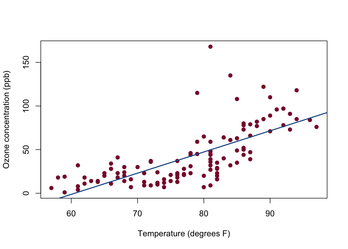
c(mean_X = mean(aq$Ozone), mean_Y = mean(aq$Temp),
  covariance = cov(aq$Ozone, aq$Temp),
  correlation = cor(aq$Ozone, aq$Temp))
## mean_X mean_Y covariance correlation
## 42.1293103 77.8706897 218.5212144 0.6983603## FALSE TRUE
## 22.55932 62.38596# Standardization and the 95% bivariate Normal ellipse
Z <- scale(aq)
D2 <- mahalanobis(Z, center = c(0, 0), cov = cov(Z))
cutoff <- qchisq(0.95, df = 2)
outside <- which(D2 > cutoff)
cbind(original_row = as.numeric(rownames(aq))[outside],
aq[outside, ], D2 = D2[outside])## original_row Ozone Temp D2
## 30 30 115 79 8.835926
## 62 62 135 84 11.326633
## 99 99 122 89 6.385194
## 117 117 168 81 25.200291# Compare real data with a fitted bivariate Normal simulation
set.seed(211)
sim <- MASS::mvrnorm(nrow(aq), mu = colMeans(aq), Sigma = cov(aq))
par(mfrow = c(1, 2))
plot(aq$Temp, aq$Ozone, pch = 19, col = "#8A1538",
xlab = "Temperature", ylab = "Ozone", main = "Observed")
plot(sim[, "Temp"], sim[, "Ozone"], pch = 19, col = "#1F5A94",
xlab = "Temperature", ylab = "Ozone", main = "Fitted Normal simulation")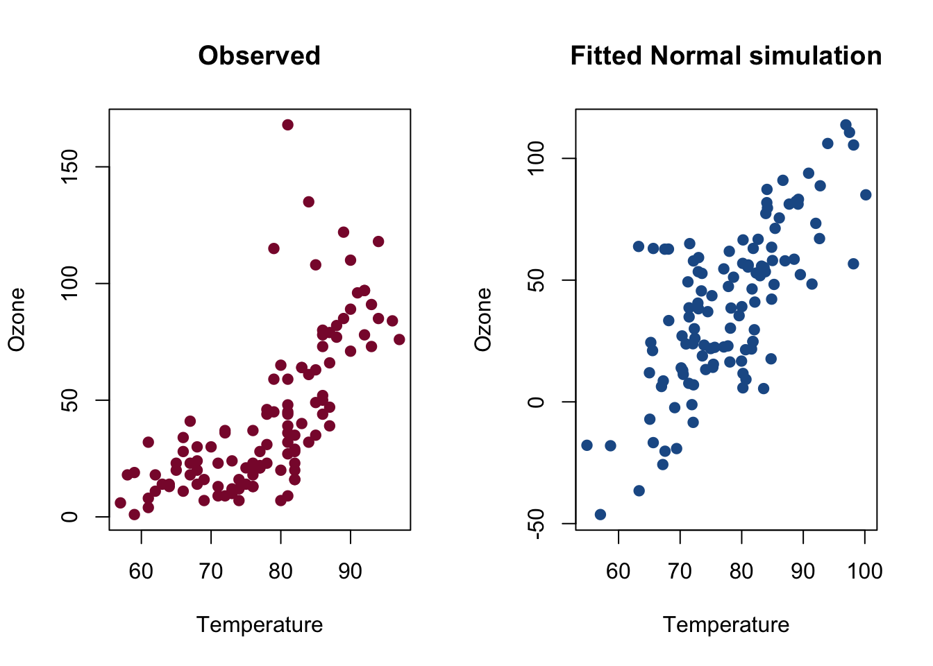
par(mfrow = c(1, 1))

# Environmental index: theoretical and empirical variance
rho <- cor(aq$Ozone, aq$Temp)
I <- 0.6 * Z[, "Ozone"] + 0.4 * Z[, "Temp"]
c(theoretical = 0.6^2 + 0.4^2 + 2 * 0.6 * 0.4 * rho,
  empirical = var(I))
## theoretical empirical
## 0.855213 0.855213The analysis is limited by missing observations, seasonal changes across May–September, possible nonlinear relations, serial dependence between neighboring days, and the right-skewed ozone distribution. These issues make the fitted bivariate Normal model informative but imperfect.
9.12 Chapter exercises
Exercise: discrete synthesis
The joint pmf of \(X,Y\in\{0,1,2\}\) is \(p_{X,Y}(x,y)=c(x+y+1)\).
- Find \(c\) and both marginal pmfs.
- Compute \(\mathbb{E}(X)\), \(\mathbb{E}(Y)\), and \(\operatorname{Cov}(X,Y)\).
- Determine whether \(X\) and \(Y\) are independent.
- Find the conditional pmf of \(X\) given \(Y=2\).
Show solution
The sum of the nine weights is \(3\sum_{x=0}^2(x+1)+3\sum_{y=0}^2y=27\), so \(c=1/27\). Summing over \(y\) gives
\[ p_X(x)=\frac{3x+6}{27}=\frac{x+2}{9}, \]
and by symmetry \(p_Y(y)=(y+2)/9\). Hence
\[ \mathbb{E}(X)=\mathbb{E}(Y) =\sum_{x=0}^2x\frac{x+2}{9}=\frac{11}{9}. \]
Also
\[ \mathbb{E}(XY) =\frac1{27}\sum_{x=0}^2\sum_{y=0}^2xy(x+y+1) =\frac{13}{9}, \]
so
\[ \operatorname{Cov}(X,Y)=\frac{13}{9}-\left(\frac{11}{9}\right)^2 =-\frac{4}{81}. \]
They are not independent; for instance, \(p(0,0)=1/27\) but \(p_X(0)p_Y(0)=4/81\). Finally, \(p_Y(2)=4/9\) and
\[ p_{X\mid Y}(x\mid2) =\frac{(x+3)/27}{4/9}=\frac{x+3}{12}, \qquad x=0,1,2. \]
Exercise: continuous synthesis
Let \(f_{X,Y}(x,y)=6y\) on \(0<y<x<1\) and zero elsewhere.
- Verify that this is a joint density.
- Find \(f_X\) and \(f_Y\).
- Find \(f_{Y\mid X}(y\mid x)\) and \(\mathbb{E}(Y\mid X=x)\).
- Compute \(\mathbb{P}(Y<X/2)\).
Show solution
First,
\[ \int_0^1\int_0^x6y\,dy\,dx =\int_0^13x^2\,dx=1. \]
The marginals are
\[ f_X(x)=\int_0^x6y\,dy=3x^2, \qquad 0<x<1, \]
and
\[ f_Y(y)=\int_y^16y\,dx=6y(1-y), \qquad 0<y<1. \]
Thus
\[ f_{Y\mid X}(y\mid x)=\frac{6y}{3x^2}=\frac{2y}{x^2}, \qquad 0<y<x, \]
and
\[ \mathbb{E}(Y\mid X=x) =\int_0^x y\frac{2y}{x^2}\,dy=\frac{2x}{3}. \]
Finally,
\[ \mathbb{P}(Y<X/2) =\int_0^1\int_0^{x/2}6y\,dy\,dx =\int_0^1\frac{3x^2}{4}\,dx=\frac14. \]
9.13 Chapter summary
- A joint distribution describes the behavior and dependence of \((X,Y)\); marginals describe the components separately.
- Expectations of functions \(g(X,Y)\) are calculated directly from the joint pmf or density.
- Covariance measures linear co-movement, while correlation standardizes it.
- Variances and covariances of sums require all relevant cross-covariance terms.
- The bivariate Normal model makes linear combinations Normal and is completely characterized by its mean vector and covariance matrix.
- Independence implies zero covariance when second moments exist, but zero covariance need not imply independence.
- Conditional distributions update uncertainty after information is observed.
- Conditional means and variances lead to the laws of total expectation and total variance.