Chapter 1 Introduction to R
1.1 Learning goals
After this chapter, you should be able to:
- recognize the R console and basic syntax;
- create and manipulate vectors, matrices, data frames, and lists;
- import and export simple data files;
- write basic functions and produce simple graphics.
1.2 Getting started
The slides introduce R as free software available for Windows, MacOS, and Linux, and present R as both a programming language and a statistical computing environment.
Try this first: type a simple command in R and press Enter.
## [1] 6## [1] 41.3 Help, libraries, and the workspace
Useful commands from the slides include help tools, demo files, and library management.
Check your understanding
What is the difference between help("plot") and library()?
help("plot") opens documentation for a specific function, while library() shows or loads installed packages.
1.4 Objects and basic data types
R works with numeric, character, and logical values. It also supports vectors, matrices, data frames, and lists.
## [1] TRUE## [1] "3"## [1] 1In R, many operations are built around objects. Once an object is created, it can be stored, transformed, printed, or reused in later commands.
1.5 Vectors and sequences
Vectors are one-dimensional collections of values. The slides emphasize the use of c(), :, seq(), and rep().
## [1] 1 4 9 2 3## [1] 1 2 3 4## [1] 1.0 1.5 2.0 2.5 3.0 3.5 4.0## [1] 1 1 1 1# simple interactive idea: change these values and re-run
start <- 2
end <- 10
step <- 2
seq(start, end, by = step)## [1] 2 4 6 8 10Mini exercise
Create a vector containing the first five odd numbers.
One solution:seq(1, 9, by = 2)
1.6 Matrices
Matrices are rectangular arrays of numbers. They can be filled by column or by row.
A <- matrix(c(2, 3, 5, 7, 11, 13), ncol = 2)
B <- matrix(c(2, 3, 5, 7, 11, 13), ncol = 2, byrow = TRUE)
A
## [,1] [,2]
## [1,] 2 7
## [2,] 3 11
## [3,] 5 13## [,1] [,2]
## [1,] 2 3
## [2,] 5 7
## [3,] 11 13## [1] 2 3 5## [1] 111.7 Data frames
A data frame stores tabular data, often with variables of different types.
students <- data.frame(
  name = c("A", "B", "C"),
  score = c(78, 85, 91),
  passed = c(TRUE, TRUE, TRUE)
)

students
## name score passed
## 1 A 78 TRUE
## 2 B 85 TRUE
## 3 C 91 TRUE## [1] 78 85 91Edit the values in students and add a new variable called grade.
1.8 Lists
A list can contain objects of different types.
## [1] "serie" "length" "type"## [1] 10## [1] 31.9 Importing and exporting data
The slides mention scan(), read.table(), write.table(), save(), load(), saveRDS(), and readRDS().
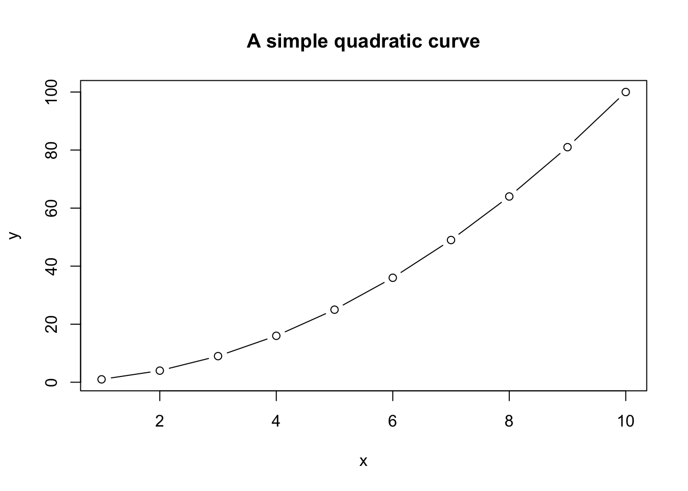
1.12 Control structures and iterations
Loops and conditional statements allow repeated computation and decision making.
## [1] 1 4 9 16 25## [1] "negative"1.13 Vectorization for probability calculations
R is designed to operate on whole vectors. Vectorized code is usually shorter, clearer, and faster than a loop.
## [1] FALSE TRUE FALSE TRUE TRUE FALSE TRUE FALSE## [1] 7## [1] 0.5Actuarial interpretation: sum(claims) is the aggregate claim count, while mean(claims > 0) is the observed proportion of policies with at least one claim.
1.14 Reproducible simulation
Random-number generators are essential in probability. set.seed() makes an experiment reproducible.
## [1] 4 6 3 5 4 2 5 6 5 5 2 3Running the chunk again with the same seed gives the same sequence. Changing or removing the seed gives a different sequence.
## [1] 0.1612## [1] 0.00372678Simulation error and model error are different. Increasing B reduces simulation error; it does not repair an unrealistic probability model.
1.15 A small probability workflow
The following pattern will recur throughout the course.
set.seed(211)
B <- 50000

# 1. Generate outcomes
x <- rbinom(B, size = 10, prob = 0.03)

# 2. Define the event
large_count <- x >= 2

# 3. Summarize
p_hat <- mean(large_count)
mcse <- sqrt(p_hat * (1 - p_hat) / B)
c(estimate = p_hat, mcse = mcse)
## estimate mcse
## 0.0331200000 0.0008002883The same three-step structure applies to market-loss events: simulate returns, define a loss threshold, and compute the proportion of simulated returns beyond the threshold.
1.16 Debugging checklist
When code fails or produces an unexpected result, check:
- capitalization (
meanandMeanare different); - unmatched parentheses or quotation marks;
- object names and dimensions (
length(),dim(),str()); - missing values (
is.na()andna.rm = TRUE); - whether a probability argument lies between 0 and 1;
- whether the random seed was set before the simulation.
Practice exercises
- Create a vector containing claim counts
0, 1, 0, 2, 1, 3. Compute its total, mean, and maximum. - Use
sample()to simulate 1,000 fair coin tosses coded as 0 and 1. Estimate the probability of heads. - Write a function
mcse(p_hat, B)that returns \(\sqrt{\hat p(1-\hat p)/B}\). - Simulate 20,000 values from a Binomial\((20,0.05)\) distribution and estimate \(\mathbb{P}(X\ge 3)\).
- Create a data frame containing policy ID, age, annual premium, and claim indicator for five fictional policies. Use logical indexing to select policies with a claim.