Chapter 6 Expectation and Other Distribution Parameters
6.1 Why summarize a distribution?
A complete pmf, pdf, or cdf contains all probabilistic information, but decisions often require a few interpretable summaries: expected cost, variability, tail percentiles, or a typical value. This chapter develops those summaries without losing sight of what each one means.
6.2 Expected value
For a discrete random variable,
\[\mathbb{E}(X)=\sum_x x p_X(x).\]
For a continuous random variable,
\[\mathbb{E}(X)=\int_{-\infty}^{\infty}x f_X(x)\,dx,\]
provided the sum or integral is absolutely convergent.
Expectation is a probability-weighted balance point and a long-run average under repeated comparable trials. It need not be a possible outcome. In actuarial work it is the pure premium before expenses, profit, and risk loadings.
Example: expected policy payment
A benefit pays QAR 0, 1,000, or 5,000 with probabilities 0.90, 0.08, and 0.02. Its expected payment is
## [1] 180The expected payment is QAR 180. This is not a possible individual payment; it is the long-run average payment per comparable policy in a large portfolio.
For constants \(a,b\) and random variables with finite expectations,
\[\mathbb{E}(aX+b)=a\mathbb{E}(X)+b.\]
More generally,
\[\mathbb{E}\!\left(\sum_{i=1}^nX_i\right)=\sum_{i=1}^n\mathbb{E}(X_i),\]
whether or not the variables are independent.
Example: expected stop-loss payment
Suppose \(X\) has density \(f_X(x)=2x\) for \(0<x<1\). A policy pays \(Y=(X-0.5)_+\). Then
\[\mathbb{E}(Y)=\int_{0.5}^{1}(x-0.5)2x\,dx=\frac{5}{24}\approx0.2083.\]
A deductible does not simply subtract 0.5 from the expected loss, because losses below the deductible produce zero payment.
## 0.2083333 with absolute error < 2.3e-156.3 Moments of a random variable
The \(k\)th raw moment is \(\mathbb{E}(X^k)\). The \(k\)th central moment is \(\mathbb{E}[(X-\mu)^k]\), where \(\mu=\mathbb{E}(X)\).
The first raw moment is the mean. The second central moment is variance. Higher central moments describe features such as asymmetry and tail weight.
The standardized third central moment measures skewness, while the standardized fourth central moment measures kurtosis. They distinguish distributions that have the same mean and variance but different asymmetry or tail behavior.
For any function \(g\) for which the expectation exists,
\[\mathbb{E}[g(X)]=\sum_xg(x)p_X(x)\]
in the discrete case, and
\[\mathbb{E}[g(X)]=\int_{-\infty}^{\infty}g(x)f_X(x)\,dx\]
in the continuous case.
Example: moments of a loaded die
For \(\mathbb{P}(X=x)=x/21\), \(x=1,\ldots,6\),
\[\mathbb{E}(X)=\sum_{x=1}^6x\frac{x}{21}=\frac{13}{3},\qquad \mathbb{E}(X^2)=\sum_{x=1}^6x^2\frac{x}{21}=21.\]
The expectation-of-a-function rule finds \(\mathbb{E}(X^2)\) directly; we do not need to derive a new distribution for \(X^2\).
6.4 Variance and standard deviation
\[\operatorname{Var}(X)=\mathbb{E}[(X-\mu)^2] =\mathbb{E}(X^2)-[\mathbb{E}(X)]^2,\]
and \(\operatorname{sd}(X)=\sqrt{\operatorname{Var}(X)}\).
Variance measures squared dispersion and is useful algebraically. Standard deviation is easier to communicate because it uses the same units as \(X\). Neither measure fully describes skewness or extreme-tail risk.
For constants \(a,b\),
\[\operatorname{Var}(aX+b)=a^2\operatorname{Var}(X).\]
For two variables,
\[\operatorname{Var}(X+Y)=\operatorname{Var}(X)+\operatorname{Var}(Y)+2\operatorname{Cov}(X,Y).\]
If \(X\) and \(Y\) are independent, their covariance is zero.
Example: same mean, different risk
x1 <- c(90, 110); p1 <- c(.5, .5)
x2 <- c(50, 150); p2 <- c(.5, .5)
c(mean1 = sum(x1*p1), sd1 = sqrt(sum((x1-100)^2*p1)),
  mean2 = sum(x2*p2), sd2 = sqrt(sum((x2-100)^2*p2)))
## mean1 sd1 mean2 sd2
## 100 10 100 50Both risks have mean 100, but the second is substantially more volatile.
Example: diversification and dependence
Two policies each have standard deviation 20. If they are independent, their total variance is \(400+400=800\). If their correlation is 0.5, their covariance is \(0.5(20)(20)=200\), and the total variance becomes
\[400+400+2(200)=1200.\]
Positive dependence weakens diversification because losses are more likely to be large together.
Example: variance of a continuous lifetime
For an exponential lifetime with rate \(\lambda\), integration gives
\[\mathbb{E}(X)=\frac1\lambda,\qquad \mathbb{E}(X^2)=\frac{2}{\lambda^2}.\]
Therefore \(\operatorname{Var}(X)=1/\lambda^2\) and \(\operatorname{sd}(X)=1/\lambda\). Unlike a bounded lifetime, the exponential model permits rare but arbitrarily large observations.
6.5 Moment generating function
The moment generating function is
\[M_X(t)=\mathbb{E}(e^{tX}),\]
when finite on an open interval containing zero. Its derivatives recover raw moments: \(M_X^{(k)}(0)=\mathbb{E}(X^k)\).
Why introduce a whole function instead of calculating moments one at a time? The MGF performs three jobs at once: its derivatives produce moments, it can identify a distribution, and multiplication converts a difficult convolution problem for independent sums into ordinary algebra:
\[M_{X+Y}(t)=M_X(t)M_Y(t).\]
An MGF packages raw moments into one function near \(t=0\). It is useful only when finite on an open interval around zero; some heavy-tailed distributions do not have an MGF for positive \(t\).
Example: Bernoulli and binomial MGFs
If \(X\sim\operatorname{Bernoulli}(p)\), then
\[M_X(t)=1-p+pe^t.\]
Therefore \(M_X'(0)=p\) and \(M_X''(0)=p\), giving \(\operatorname{Var}(X)=p(1-p)\). If \(S=X_1+\cdots+X_n\) is a sum of independent Bernoulli variables, then
\[M_S(t)=[1-p+pe^t]^n,\]
the MGF of a binomial distribution.
Motivation example: total continuous waiting time
Let \(X_1,\ldots,X_n\) be independent exponential waiting times with common rate \(\lambda\). Since
\[M_{X_i}(t)=\frac{\lambda}{\lambda-t},\qquad t<\lambda,\]
the total waiting time \(T=\sum_iX_i\) has
\[M_T(t)=\left(\frac{\lambda}{\lambda-t}\right)^n.\]
This is the MGF of a gamma distribution with shape \(n\) and rate \(\lambda\). Thus the MGF identifies the law of the sum without deriving its density by repeated integration. It also gives \(\mathbb{E}(T)=n/\lambda\) and \(\operatorname{Var}(T)=n/\lambda^2\).
6.6 Characteristic function
The MGF is convenient but may be infinite away from zero—for example, for some heavy-tailed losses. A characteristic function replaces \(e^{tX}\) by the bounded complex number \(e^{itX}\). We need it when we want a transform that exists for every distribution, uniquely identifies that distribution, and still turns independent sums into products. It is also the main transform used to prove convergence in distribution and central limit results.
The characteristic function of \(X\) is
\[\varphi_X(t)=\mathbb{E}(e^{itX}) =\mathbb{E}[\cos(tX)]+i\mathbb{E}[\sin(tX)],\qquad t\in\mathbb{R},\]
where \(i^2=-1\).
Every random variable has a characteristic function, \(\varphi_X(0)=1\), and \(|\varphi_X(t)|\le1\). For independent \(X\) and \(Y\),
\[\varphi_{X+Y}(t)=\varphi_X(t)\varphi_Y(t).\]
When the relevant moments exist,
\[\varphi_X^{(k)}(0)=i^k\mathbb{E}(X^k).\]
The characteristic function uniquely determines the distribution and always exists. It is especially useful for studying sums and convergence when an MGF is unavailable.
Example: a Bernoulli characteristic function
For \(X\sim\operatorname{Bernoulli}(p)\),
\[\varphi_X(t)=1-p+pe^{it}.\]
Since \(\varphi_X'(0)=ip\), we recover \(\mathbb{E}(X)=\varphi_X'(0)/i=p\).
Example: a normal characteristic function
If \(X\sim N(\mu,\sigma^2)\), then
\[\varphi_X(t)=\exp\!\left(i\mu t-\frac{\sigma^2t^2}{2}\right).\]
Multiplying characteristic functions of independent normal variables adds their means and variances, showing immediately that their sum is normal.
t <- seq(-8, 8, length.out = 401)
phi <- exp(-t^2 / 2)
plot(t, phi, type = "l", lwd = 3, col = "#8A1538",
     xlab = "t", ylab = expression(phi[X](t)))
abline(h = 0, col = "grey70")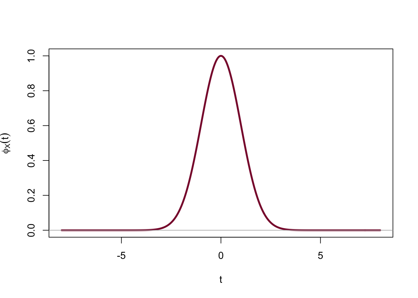
Motivation example: a heavy-tailed continuous variable
For a standard Cauchy variable, \(\mathbb{E}(e^{tX})\) is not finite for any nonzero real \(t\), so an MGF cannot be used. Its characteristic function nevertheless exists:
\[\varphi_X(t)=e^{-|t|}.\]
For independent standard Cauchy variables \(X_1\) and \(X_2\),
\[\varphi_{X_1+X_2}(t)=e^{-2|t|},\]
which identifies their sum as Cauchy with scale 2. The example shows why characteristic functions are more universal than MGFs. Notice also that the cusp at zero is consistent with the Cauchy distribution not having a finite mean.
6.7 Probability generating function
For a nonnegative integer-valued random variable, the probability generating function is
\[G_X(s)=\mathbb{E}(s^X)=\sum_{x=0}^{\infty}p_X(x)s^x.\]
Why use a separate transform for counts? Because its power-series coefficients are the probabilities themselves. The coefficient of \(s^x\) is \(p_X(x)\), while \(G_X'(1)=\mathbb{E}(X)\) and \(G_X''(1)=\mathbb{E}[X(X-1)]\). Products describe sums of independent counts, and composition describes random sums and branching processes. A PGF is therefore more directly interpretable for counts than an MGF, but it is not designed for general continuous variables.
Example: Bernoulli PGF
If \(X\sim\operatorname{Bernoulli}(p)\), then \(G_X(s)=1-p+ps\). Consequently \(G_X'(1)=p\), as expected.
Example: Poisson PGF and factorial moments
If \(N\sim\operatorname{Poisson}(\lambda)\), then
\[G_N(s)=\exp\{\lambda(s-1)\}.\]
Thus \(G_N'(1)=\lambda\) and \(G_N''(1)=\lambda^2\). Consequently,
\[\operatorname{Var}(N)=G_N''(1)+G_N'(1)-[G_N'(1)]^2=\lambda.\]
PGF derivatives naturally produce factorial moments, making them especially effective for claim-count models.
Motivation example: a random number of arrivals
Suppose each of \(n\) independently contacted customers responds with probability \(p\). Each response indicator has PGF \(1-p+ps\), so the total response count has
\[G_N(s)=(1-p+ps)^n.\]
Expanding the polynomial immediately reveals every count probability. More generally, if a system produces a random number of offspring and repeats independently, composing the PGF tracks the population across generations—one reason PGFs are fundamental in branching-process models.
6.8 Percentiles
A \(p\)th quantile is a value
\[q_p=\inf\{x:F_X(x)\ge p\},\qquad 0<p<1.\]
The 95th percentile is a threshold that the variable does not exceed with probability at least 0.95. In risk management it describes a tail threshold, whereas the mean describes a center.
## [1] 0.000000 1.281552 1.644854 2.3263486.9 Median and mode
The median is a 50th percentile. It is resistant to a small number of extreme observations. A mode is a value at which the pmf or pdf is maximized.
Mean, median, and mode answer different questions. For a right-skewed loss distribution the mode is often below the median, which is below the mean. No single measure is always the “best” center.
6.10 Chebyshev’s inequality
If \(X\) has mean \(\mu\) and finite variance \(\sigma^2\), then for every \(k>0\),
\[\mathbb{P}(|X-\mu|\ge k\sigma)\le\frac{1}{k^2}.\]
Equivalently, for \(k>1\),
\[\mathbb{P}(|X-\mu|<k\sigma)\ge1-\frac{1}{k^2}.\]
Chebyshev’s inequality needs no distributional shape assumption. Its price for being universal is that the bound can be conservative. It is a guaranteed minimum, not a prediction that equality will hold.
Example
If a portfolio loss has mean 2 million and standard deviation 0.3 million, then at least \(1-1/3^2=8/9\) of outcomes lie between 1.1 and 2.9 million.
This is a guaranteed lower bound, not an assertion that exactly \(8/9\) of losses lie there. When the full distribution is known, the actual probability may be considerably larger.
Exercises
Exercise 1: moments
For \(X\) with values \(0,1,2\) and probabilities \(0.2,0.5,0.3\), calculate \(\mathbb{E}(X)\), \(\mathbb{E}(X^2)\), variance, and standard deviation.
Show solution
\(\mathbb{E}(X)=1.1\), \(\mathbb{E}(X^2)=1.7\), \(\operatorname{Var}(X)=1.7-1.1^2=0.49\), and \(\operatorname{sd}(X)=0.7\).Exercise 2: transformation
If \(Y=500+1.2X\), \(\mathbb{E}(X)=1000\), and \(\operatorname{Var}(X)=40{,}000\), find the mean and variance of \(Y\).
Show solution
\(\mathbb{E}(Y)=500+1.2(1000)=1700\) and \(\operatorname{Var}(Y)=1.2^2(40{,}000)=57{,}600\).Exercise 3: quantile
If \(F(x)=1-e^{-x/100}\) for \(x\ge0\), find the 95th percentile.
Show solution
Solve \(1-e^{-q/100}=0.95\), giving \(q=-100\log(0.05)\approx299.57\).Exercise 4: Chebyshev
A loss has mean 80 and variance 100. Give a guaranteed lower bound for \(\mathbb{P}(50<X<110)\).
Show solution
The interval is within three standard deviations of the mean. Chebyshev gives at least \(1-1/9=8/9\).Exercise 5: expected insurance payment
A loss \(X\) equals 0, 500, and 2,000 with probabilities 0.70, 0.20, and 0.10. A policy pays \(Y=(X-300)_+\). Find \(\mathbb{E}(X)\) and \(\mathbb{E}(Y)\).
Show solution
\[\mathbb{E}(X)=0(.7)+500(.2)+2000(.1)=300.\]
The possible payments are 0, 200, and 1,700, so
\[\mathbb{E}(Y)=0(.7)+200(.2)+1700(.1)=210.\]Exercise 6: variance of a portfolio
Losses \(X\) and \(Y\) have standard deviations 10 and 20 and correlation 0.25. Find \(\operatorname{Var}(X+Y)\). What would it be under independence?
Show solution
\(\operatorname{Cov}(X,Y)=0.25(10)(20)=50\). Hence
\[\operatorname{Var}(X+Y)=10^2+20^2+2(50)=600.\]
Under independence the covariance is zero, giving 500.Exercise 7: an MGF
Suppose \(M_X(t)=\exp\{3(e^t-1)\}\). Find \(\mathbb{E}(X)\) and \(\operatorname{Var}(X)\).
Show solution
\(M_X'(0)=3\) and \(M_X''(0)=12\). Therefore
\[\operatorname{Var}(X)=12-3^2=3.\]
This is the MGF of a Poisson variable with parameter 3.Exercise 8: characteristic function
Let \(X\) equal \(-1\) and 1 with equal probability. Find \(\varphi_X(t)\) and use it to obtain \(\mathbb{E}(X)\) and \(\mathbb{E}(X^2)\).
Show solution
\[\varphi_X(t)=\frac{e^{-it}+e^{it}}2=\cos t.\]
Since \(\varphi_X'(0)=0=i\mathbb{E}(X)\), \(\mathbb{E}(X)=0\). Also \(\varphi_X''(0)=-1=i^2\mathbb{E}(X^2)\), so \(\mathbb{E}(X^2)=1\).Exercise 9: PGF and probability extraction
Suppose \(G_X(s)=(0.7+0.3s)^3\). Identify the distribution, find \(\mathbb{P}(X=2)\), and calculate \(\mathbb{E}(X)\).
Show solution
\(X\sim\operatorname{Binomial}(3,0.3)\). The coefficient of \(s^2\) is
\[\binom32(0.3)^2(0.7)=0.189,\]
and \(\mathbb{E}(X)=G_X'(1)=0.9\).Exercise 10: median and mean
A loss has cdf \(F(x)=1-e^{-x/50}\) for \(x\ge0\). Find its median and compare it with its mean, which is 50.
Show solution
The median satisfies \(1-e^{-m/50}=0.5\), so
\[m=50\log2\approx34.66.\]
The median is below the mean, consistent with a right-skewed loss distribution.Exercise 11: continuous moments and variance
Let \(X\) have density \(f(x)=3x^2\) for \(0<x<1\). Find \(\mathbb{E}(X)\), \(\mathbb{E}(X^2)\), and \(\operatorname{Var}(X)\).
Show solution
\[\mathbb{E}(X)=\int_0^1 3x^3\,dx=\frac34,qquad \mathbb{E}(X^2)=\int_0^1 3x^4\,dx=\frac35.\]
Thus \(\operatorname{Var}(X)=3/5-(3/4)^2=3/80\).Exercise 12: continuous MGF and a sum
Independent variables \(X_1,X_2\) are exponential with rate 2. Use MGFs to identify the distribution of \(S=X_1+X_2\) and find its mean and variance.
Show solution
\(M_X(t)=2/(2-t)\), so \(M_S(t)=[2/(2-t)]^2\). This is the MGF of \(\operatorname{Gamma}(2,2)\). Hence \(\mathbb{E}(S)=2/2=1\) and \(\operatorname{Var}(S)=2/2^2=1/2\).Exercise 13: continuous characteristic function
Let \(X\sim N(2,9)\). Write its characteristic function. If \(Y\sim N(-1,4)\) is independent of \(X\), use characteristic functions to identify \(X+Y\).
Show solution
\[\varphi_X(t)=\exp(2it-9t^2/2),\qquad \varphi_Y(t)=\exp(-it-4t^2/2).\]
Their product is \(\exp(it-13t^2/2)\), the characteristic function of \(N(1,13)\).Exercise 14: continuous percentile and Chebyshev
A continuous lifetime has mean 100 hours and standard deviation 10 hours. (a) Without assuming a distribution, give a lower bound for \(\mathbb{P}(70<X<130)\). (b) If it is normal, find the actual probability approximately.
Show solution
- The interval is within three standard deviations, so Chebyshev gives at least \(8/9\approx0.8889\). (b) Under normality, the probability is \(\Phi(3)-\Phi(-3)\approx0.9973\). This comparison illustrates why Chebyshev is safe but conservative.
6.11 Chapter summary
Expectation describes long-run center; moments and variance describe distributional shape and dispersion. MGFs, characteristic functions, and PGFs encode distributions and simplify the study of moments and sums. Quantiles, medians, and modes offer alternative summaries, while Chebyshev’s inequality gives distribution-free probability guarantees.