Chapter 7 Frequently Used Discrete Distributions
7.1 Choosing a discrete model
A named distribution is not merely a formula. It is a compact statement about how the data are generated. Before calculating, ask whether the variable counts successes, waits for a success, counts events in exposure, or samples without replacement.
Use the interactive explorers to change parameters and compare two models. Each explorer displays the pmf and cdf side by side, so changes in probability mass and cumulative probability remain connected.
7.2 Discrete uniform distribution
Why it is useful—two applications. (1) The score on a fair die or the selected integer from a properly designed random-number generator has equally likely values. (2) In randomized experiments, a treatment label chosen uniformly from a finite list models a transparent allocation mechanism. Use this family only when the mechanism genuinely makes all listed outcomes equally likely.
If \(X\) is equally likely to take each integer \(a,a+1,\ldots,b\), then
\[\mathbb{P}(X=x)=\frac{1}{b-a+1},\]
with \(\mathbb{E}(X)=(a+b)/2\) and \(\operatorname{Var}(X)=((b-a+1)^2-1)/12\).
This model is appropriate only when symmetry or the mechanism justifies equally likely values—for example, a fair die.
x <- 1:6
plot(x, rep(1/6, 6), type = "h", lwd = 6, col = "#8A1538",
     xlab = "x", ylab = "Probability", main = "Fair die")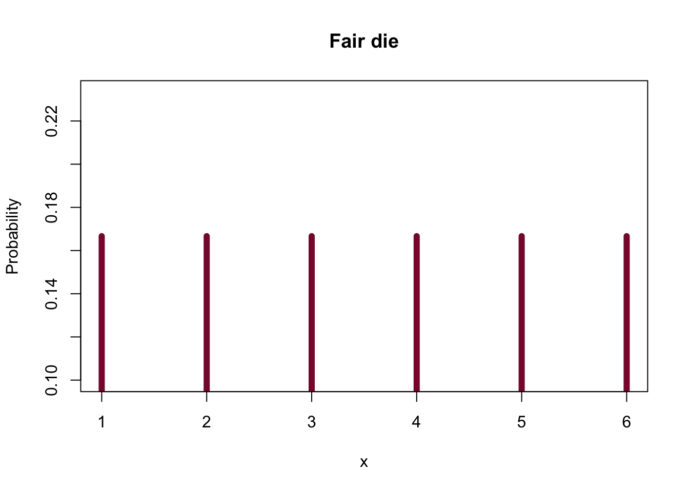
Move the lower and upper integer endpoints to see how widening the support lowers every probability mass and stretches the cdf across more steps.
7.3 Bernoulli distribution
Why it is useful—two applications. (1) Record whether a manufactured item passes inspection. (2) Record whether a website visitor clicks a particular link. Many larger count models begin by coding each elementary yes/no outcome as a Bernoulli variable.
\(X\sim\operatorname{Bernoulli}(p)\) records one success/failure trial:
\[\mathbb{P}(X=x)=p^x(1-p)^{1-x},\quad x=0,1.\]
Its mean is \(p\) and variance is \(p(1-p)\).
A Bernoulli variable can represent whether one policy has a claim, one loan defaults, or one transaction is fraudulent.
7.4 Binomial distribution
Why it is useful—two applications. (1) Count germinating seeds among \(n\) independently planted seeds under common conditions. (2) Count correct answers among \(n\) independent true/false questions when the success probability is stable. The model is useful because it aggregates repeated Bernoulli trials into one count.
\(X\sim\operatorname{Binomial}(n,p)\) counts successes in \(n\) independent Bernoulli trials having the same success probability \(p\):
\[\mathbb{P}(X=x)=\binom nxp^x(1-p)^{n-x},\quad x=0,\ldots,n.\]
\(\mathbb{E}(X)=np\) and \(\operatorname{Var}(X)=np(1-p)\).
The factor \(\binom nx\) counts which trials produced the \(x\) successes. Check all three assumptions: fixed \(n\), common \(p\), and independence. Heterogeneous risks or contagion can invalidate the model.
Example: claim indicators
For 20 independent policies, suppose each policy has probability \(0.05\) of producing a claim during the year. Define the indicator \(I_i=1\) when policy \(i\) produces a claim and \(I_i=0\) otherwise. The total number of policies with claims is
\[X=I_1+\cdots+I_{20}\sim\operatorname{Bin}(20,0.05).\]
Two useful portfolio questions are the probability of no claims and the probability of at least two claims:
\[\mathbb{P}(X=0)=(0.95)^{20},\qquad \mathbb{P}(X\ge 2)=1-\mathbb{P}(X=0)-\mathbb{P}(X=1).\]
##    no_claims at_least_two
##    0.3584859    0.2641605
Thus, the probability of a claim-free portfolio is approximately \(0.3585\), while the probability that at least two policies generate claims is approximately \(0.2642\). The model turns many individual yes/no outcomes into one count, which is exactly the role of the binomial distribution.
7.5 Poisson distribution
Why it is useful—two applications. (1) Count calls reaching a help desk during a fixed hour. (2) Count meteor impacts, mutations, or flaws per fixed region when events are rare and approximately independent. The exposure may be time, distance, area, or volume—not only a clock interval.
\(X\sim\operatorname{Poisson}(\lambda)\) models an event count in fixed exposure:
\[\mathbb{P}(X=x)=e^{-\lambda}\frac{\lambda^x}{x!},\quad x=0,1,\ldots,\]
and \(\mathbb{E}(X)=\operatorname{Var}(X)=\lambda\).
The model is motivated by events occurring independently at a stable average rate. The equality of mean and variance is diagnostic: substantial overdispersion suggests heterogeneity or clustering.
The law of rare events: Poisson approximation to the binomial
The Poisson distribution also appears as the limiting model for a large number of independent opportunities, each having a very small chance of success. This setting is common when counting rare defects, unusual mutations, system failures, or uncommon responses in a large population.
Let \(X_n\sim\operatorname{Binomial}(n,p_n)\). If
\[p_n\longrightarrow0,\qquad n\longrightarrow\infty,qquad np_n\longrightarrow\lambda<\infty,\]
then, for every fixed nonnegative integer \(k\),
\[\mathbb{P}(X_n=k)\longrightarrow e^{-\lambda}\frac{\lambda^k}{k!}.\]
Thus \(X_n\) converges in distribution to \(\operatorname{Poisson}(\lambda)\).
The condition \(np_n\to\lambda\) keeps the expected number of events finite even though the number of opportunities grows. Starting from the binomial pmf,
\[\binom nkp_n^k(1-p_n)^{n-k},\]
the factor \((1-p_n)^n\) approaches \(e^{-\lambda}\), while the remaining factors approach \(\lambda^k/k!\).
Example: rare manufacturing defects
Suppose 2,000 independently produced chips each have defect probability \(0.0008\). If \(X\) is the number of defective chips, then
\[X\sim\operatorname{Binomial}(2000,0.0008),\qquad np=1.6.\]
The Poisson approximation uses \(Y\sim\operatorname{Poisson}(1.6)\). For the probability of at least two defects,
n <- 2000; p <- .0008; lambda <- n*p
c(exact_binomial = 1 - pbinom(1, n, p),
  poisson_approximation = 1 - ppois(1, lambda))
## exact_binomial poisson_approximation
## 0.4751466 0.4750691The approximation avoids a large binomial calculation and makes the expected rare-event count \(\lambda=np\) explicit.
Chen’s formula (Poisson identity)
If \(X\sim\operatorname{Poisson}(\lambda)\) and the expectations exist, then for any suitable function \(g\),
\[\mathbb{E}[Xg(X)]=\lambda\,\mathbb{E}[g(X+1)].\]
This identity, often called the Poisson Chen–Stein identity, characterizes the Poisson distribution and provides a quick way to calculate moments. It follows by shifting the index in the Poisson sum:
\[\sum_{x=0}^{\infty}xg(x)e^{-\lambda}\frac{\lambda^x}{x!} =\lambda\sum_{y=0}^{\infty}g(y+1)e^{-\lambda}\frac{\lambda^y}{y!}.\]
Example: obtaining Poisson moments from Chen’s formula
Take \(g(x)=1\). Then
\[\mathbb{E}(X)=\lambda.\]
Next take \(g(x)=x\). Chen’s formula gives
\[\mathbb{E}(X^2)=\lambda\mathbb{E}(X+1) =\lambda(\lambda+1)=\lambda^2+\lambda.\]
Therefore
\[\operatorname{Var}(X)=\mathbb{E}(X^2)-[\mathbb{E}(X)]^2=\lambda.\]
The same technique can generate higher moments by choosing \(g(x)=x^2,x^3,\ldots\).
7.6 Geometric distribution
Why it is useful—two applications. (1) Count attempts until a student first solves a randomly generated puzzle of fixed difficulty. (2) Count inspected components until the first defective one appears when successive outcomes are independent with constant defect probability. Its memorylessness makes it appropriate only when previous failures do not change the next success chance.
If \(X\) is the trial number of the first success in independent Bernoulli trials, then
\[\mathbb{P}(X=x)=(1-p)^{x-1}p,\quad x=1,2,\ldots,\]
with \(\mathbb{E}(X)=1/p\) and \(\operatorname{Var}(X)=(1-p)/p^2\).
The geometric distribution is memoryless: \(\mathbb{P}(X>s+t\mid X>s)=\mathbb{P}(X>t)\). Waiting longer does not change the future waiting distribution when \(p\) remains constant.
7.7 Negative binomial distribution
Why it is useful—two applications. (1) Count unsuccessful attempts before a player achieves a specified number of wins. (2) Model biological or ecological event counts whose variability exceeds their mean; unobserved differences between subjects can produce this overdispersion. These two applications reflect its waiting-time and flexible count-model interpretations.
In the convention used by R, \(X\sim\operatorname{NegBin}(r,p)\) counts failures before the \(r\)th success:
\[\mathbb{P}(X=x)=\binom{x+r-1}{x}p^r(1-p)^x,\quad x=0,1,\ldots\]
\(\mathbb{E}(X)=r(1-p)/p\) and \(\operatorname{Var}(X)=r(1-p)/p^2\).
Always state whether the variable counts trials or failures; the two conventions differ by \(r\). In count modeling, the negative binomial also offers variance larger than its mean.
7.8 Hypergeometric distribution
Why it is useful—two applications. (1) Count marked fish in a sample drawn without replacement during a capture–recapture study. (2) Count defective chips in a quality-control sample taken from a finite shipment. It replaces the binomial whenever sampling materially changes what remains in the population.
From a population of \(N\) objects containing \(K\) successes, sample \(n\) objects without replacement. If \(X\) counts sampled successes,
\[\mathbb{P}(X=x)=\frac{\binom Kx\binom{N-K}{n-x}}{\binom Nn}.\]
Unlike the binomial model, draws are dependent because removing an object changes the population composition. This is the natural model for audits and quality-control sampling from finite inventories.
## [1] 0.67433077.9 Summary of discrete distributions
| Distribution | What it models | Parameters | Mean | Variance |
|---|---|---|---|---|
| Discrete uniform | Equally likely integers | \(a,b\) | \((a+b)/2\) | \(((b-a+1)^2-1)/12\) |
| Bernoulli | One success indicator | \(p\) | \(p\) | \(p(1-p)\) |
| Binomial | Successes in fixed independent trials | \(n,p\) | \(np\) | \(np(1-p)\) |
| Poisson | Events in fixed exposure | \(\lambda\) | \(\lambda\) | \(\lambda\) |
| Geometric | Trial of first success | \(p\) | \(1/p\) | \((1-p)/p^2\) |
| Negative binomial | Failures before \(r\)th success | \(r,p\) | \(r(1-p)/p\) | \(r(1-p)/p^2\) |
| Hypergeometric | Successes without replacement | \(N,K,n\) | \(nK/N\) | \(n(K/N)(1-K/N)(N-n)/(N-1)\) |
Exercises
Exercise 1: model selection
Choose a distribution for: (a) claims among 100 similar independent policies; (b) claims arriving during one hour at a stable rate; (c) erroneous files among 12 selected without replacement from 80 files.
Show solution
- Binomial, (b) Poisson, and (c) Hypergeometric.
Exercise 2: binomial
If \(X\sim\operatorname{Binomial}(10,0.2)\), find \(\mathbb{P}(X\ge2)\).
Show solution
\[1-\mathbb{P}(X=0)-\mathbb{P}(X=1)=1-0.8^{10}-10(0.2)(0.8)^9\approx0.6242.\]Exercise 3: Poisson
Monthly claims follow a Poisson distribution with mean 4. Find the probability of exactly 3 claims and of more than 5.
7.10 Chapter summary
The data-generating mechanism selects the distribution. Fixed independent trials suggest binomial; stable-rate event counts suggest Poisson; waiting for successes suggests geometric or negative binomial; and sampling without replacement suggests hypergeometric. Parameter changes should be interpreted through both the pmf and cdf.